22 Exoplanets: Statistics and Modern Discoveries
The existence of planets around other stars is now commonplace — over 5,000 exoplanets have been detected in 2023 compared to less than 50 known exoplanets in 2000. That’s a 100-fold increase in just over 20 years! The solar systems that have been found look very different from our own. Some have gas giants orbiting very close to their host stars and others have planets with sizes that are not seen amongst our eight planets. Let’s take a look at the diversity of planets and planetary systems that have been found and highlight a few of the most interesting, with respect to the possibility of finding life.
Learning Objectives
By the end of this chapter, you will be able to:
- Discuss the ranges for mass and radius that the exoplanets discovered have
- Describe the types of exoplanets being detected and how they compare to the planets in our solar system
- Explain how different detection techniques are sensitive to detecting different kinds of exoplanets.
- Discuss the TRAPPIST-1 planetary system and how it is similar to and different from our own
Exoplanet Statistics
Now that a large sample of exoplanets have been detected, we can take stock of the types of planets that have been found. Overall, the transit method and radial velocity methods have yielded the most exoplanets to date, with 75% of known exoplanets found with the transit method and 19% with the radial velocity method. The animation below summarizes the history of planetary discovery. Note the explosion of detections with the transit method in 2014 when data from the Kepler mission started coming in.
Timeline for exoplanet discoveries.
Figures 1 and 2 below summarize the detections by the plotting the planet’s mass (Fig. 1) and the planet’s radius (Fig. 2) against how long it takes the planet to orbit its host star (its period). Each planet has a symbol to indicate which detection method was used to discover the exoplanet. There are two methods included in Figures 1 and 2 which we did not discuss in the previous chapter, as neither are one of the primary methods used: timing variations and orbital brightness modulations. We’ll explain these two methods briefly.
When and for how long a planetary transit will occur is predictable. If there is another unseen planet in the system that is gravitationally tugging on the transiting exoplanet, this can cause the transiting planet to either speed up or slow down and it will cross in front of the star sooner or later than predicted. This is the theory behind timing variations. This method has the advantage of allowing you to determine the mass of the exoplanets. A couple dozen of the more than 5,000 exoplanets detected to date were found via timing variations. In our own solar system, the planet Neptune was discovered via timing variations in 1846 — Uranus was found to orbit slower or faster during its orbit around the Sun than predicted, and the presence of another planet was hypothesized to be the reason. Neptune was found exactly where it would be if it was the cause for the changes in Uranus’ orbital motion. Science!
A massive planet orbiting very close to its host star can cause the brightness of the star to change due changes in the amount of light reflecting off the planet’s surface. Of course, the planet needs to have a reflective surface for this effect to be measured, and these changes in reflected light will manifest as a change in the brightness of the star that is in lockstep with the orbital period (or phases) of the close-in planet. These types of changes are called orbital brightness modulations. Changes in brightness can also be caused by distortions to the star’s shape caused by the massive, close-orbiting planet.
There a few important limitations to Figures 1 and 2 that we need to note. Figure 1 shows the mass and orbital period of the exoplanets. The mass of an exoplanet can be found with the radial velocity (RV) method and the timing variations method. The transit method allows you to determine the radius of an exoplanet but not the mass. Not all exoplanets found with the transit method have been followed up with the RV method to get the mass, so not all planets found with the transit method are included in Figure 1.
In a similar way, not all exoplanets detected with the RV method are shown in Figure 2, and this is clear to see as Figure 2 is dominated by green squares for the transit method. Of the 1000+ stars found with the RV method, only the 66 that have had their radii determined are included in Figure 2.


Concept Check: Analyzing the Mass-Period and Radius-Period Plots
There are trends in the mass-period plot in Figure 1 that are especially prevalent when looking at the distribution for each detection method.
Transit Method
What trends do you see in radius and period for the exoplanets found using the transit method?
Looking at the radius-period plot (Figure 2), the transit method overwhelmingly finds planets with periods less than a hundred days. There are very few exoplanets found with periods greater than the Earth (365 days) — the limit is about 1,000 days which is a little less than 3 Earth years.
The transit method picks up planets with a wide range of radii, from planets smaller than the Earth all the way up to planets 30 times larger than the Earth. However, intuitively, planets with very small radii will be the most difficult to detect, as these cause the least amount of dimming in the brightness of the host star.
Summary: Most radii, short periods (a few hours up to a few years).
What types of exoplanets will the transit method preferentially detect?
The transit method is best at finding exoplanets that are fairly close to their host stars. This is not a technical fault of the method itself but rather the fact that to collect data for planets on long period orbits, you need measurements spanning decades or centuries, and we’ve only been observing transits for about 20 years so far.
Radial Velocity Method
What trends do you see in mass and period for the exoplanets found using the radial velocity (RV) method?
The RV method is able to find exoplanets with a wide range of orbital periods, from less than 1 day up to 105 days (275 years). The method is sensitive to a wide range of masses, from planets slightly less-massive than the Earth up to planets with 30 times the mass of Jupiter; there are more higher mass planets found than lower mass planets. As for the period range, there is a generally diagonal trend, where low-mass planets with shorter orbital periods and high-mass planets with longer orbital periods are found. There is some scatter whereby higher-mass planets with shorter orbital periods are found, but virtually no planets with lower masses and periods greater than 1 year are detected.
What types of exoplanets will the RV method preferentially detect? What are the limitations?
The RV method is best at finding massive planets with periods out to about 50 years. The method can also find lower mass planets orbiting close to their host stars but cannot detect low-mass planets orbiting further away.
Direct Imaging
What trends do you see in mass and period for the exoplanets found using the imaging method? How about trends in the radius and period?
What types of exoplanets will the direct imaging method preferentially detect?
Gravitational Microlensing
What trends do you see in mass and period for the exoplanets found using the microlensing method? Why do you think the radius cannot be determined for the microlensing method (that is, why is this method not shown in the radius-period plot)?
What types of exoplanets will gravitational microlensing preferentially detect?
In Figure 2, there is a gap for planets with radii of 4 to 10 times the radius of the Earth (4 REarth < R < 10 REarth), especially for planets that are orbiting close to their host stars. There are Jupiter-sized planets found orbiting close to their stars (hot Jupiters) as well as Earth-sized planets orbiting close — where are the planets with radii 4-10 REarth? Is this gap due to limitations of the detection methods or is this telling us something more general about the types of planets that form around stars? Since the transit method can detect stars below and above this range of radii, this suggests the gap (sometimes called the “hot Neptune desert”) is real and that it has something to do either with the formation or longevity of planets this size. One idea is that planets of this size are most susceptible to having their atmospheres completely evaporate away, making them planets that can transition in size and eventually have a smaller radius (where planets are found).
The types of planets being found are commonly divided into four main categories: gas giants, Neptune-like, super-Earths, and terrestrial. Figure 3 summarizes the fraction of each of these types that has been found. Super-Earths have radii between 1.2 and 2.8 that of Earth, and the other large group with sizes between 2.8 and 4 that of Earth are often called Neptune-like or mini-Neptunes. While the totals are split into about one-third each for gas giants, super-Earths, and Neptune-like exoplanets, we need to keep in mind that the transit method, which has found 75% of all exoplanets, is biased against very small, terrestrial-size planets. The smallest radius for an exoplanet detected with the transit method is about 30% the size of Earth’s radius (R = 0.30 REarth), so we cannot immediately conclude that there are fewer terrestrial exoplanets out there compared to the other types. In our own solar system, two of the eight planets, Mercury and Mars, have radii of 0.39 REarth and 0.53 REarth.

For a clearer look into the distribution of exoplanets by their size, Figure 4 shows a histogram of the radii for known transiting exoplanets that have a measured radius. This does not eliminate the bias against terrestrial planets but some interesting trends emerge.

First, we see a preponderance of exoplanets with sizes intermediate between the Earth and Neptune — the super-Earths and mini-Neptunes. No planets of these types exist in our solar system! What a remarkable discovery it is that the most common types of planets in the Galaxy are completely absent from our solar system and were unknown until the Kepler mission. Further, this idea that planets of roughly Earth’s size are so numerous is surely one of the most important discoveries of modern astronomy.
The TRAPPIST-1 system
One of the most intriguing planetary systems detected so far is TRAPPIST-1. The TRAPPIST-1 planetary system is about 40 light years away from Earth and has seven known exoplanets. The TRAPPIST-South survey program came online in 2010 by European astronomers using a small, ground-based telescope at La Silla Observatory in Chile to search for exoplanets with the transit method. The acronym TRAPPIST stands for “Transiting Planets and Planetesimals Small Telescope,” and is a nod to the popular Trappist beers found in Belgium.
In 2015, three planets were detected with this survey around a star that the team renamed TRAPPIST-1 (catchier than the original catalog name for this star, 2MASS J23062928-0502285). TRAPPIST-1 is a small, cool, red dwarf; the advantage of looking at small stars is that the transit signals from smaller, terrestrial planets are stronger. In 2017, four more planets were discovered around TRAPPIST-1, with the transit timing variations, bringing the total to seven planets orbiting TRAPPIST-1. All of these planets orbit at a distance that is smaller than the distance from the Sun to Mercury in our solar system and are similar in size to the rocky terrestrial worlds. Figure 5 below summarizes the properties of the seven known planets orbiting TRAPPIST-1 compared to our solar system’s four terrestrial planets.

Worked Example: Finding an Exoplanet’s Density
If both the mass and radius are known for an exoplanet, we can find its density. We explored this quantitatively in the chapter on the Earth but revisit it here with an emphasis on finding densities for exoplanets.
Notice that the masses and radii for the TRAPPIST-1 planets are reported relative to the Earth. For example, TRAPPIST-1 b has a radius that is 12% larger than the Earth’s radius (RT1b = 1.12 REarth) and a mass almost identical to the Earth’s (MT1b = 1.02 MEarth). Since these values are relative to the Earth, we can immediately estimate TRAPPIST-1 b’s density:
[latex]\rho = M/V = M/\frac{4}{3} \pi R^3[/latex]
Now, by taking the ratio of the density of any exoplanet to that of the Earth’s density, we can find the density of the exoplanet relative to Earth:
[latex]\rho/\rho_{E} = (M/\frac{4}{3} \pi R^3)/(M_{E}/\frac{4}{3} \pi R_{E}^3) = (M/M_{E})/(R/R_{E})^3[/latex]
Putting in the values of the mass and radius for TRAPPIST-1 b, we find:
ρT1b = (1.02 MEarth/MEarth)/(1.12 REarth/REarth)3 ρEarth = (1.02)/(1.12)3 ρEarth = 0.73 ρEarth
This agrees perfectly with the value reported in Figure 5.
Question 1
The exoplanet 51 Peg b has a radius that is 1.27 times greater than Jupiter’s radius (R51P = 1.27 RJ) and a mass that is 0.46 (46%) the mass of Jupiter (M51Pb = 0.46 MJ). Find the density of 51 Peg b relative to Jupiter’s density.
Show Answer
This can be solved exactly the same way as the example above (the only difference is that the mass and radius are now reported relative to Jupiter, rather than Earth).
[latex]\rho/\rho_{J} = (M/\frac{4}{3} \pi R^3)/(M_{J}/\frac{4}{3} \pi R_{J}^3) = (M/M_{J})/(R/R_{J})^3[/latex]
Putting in the values of the mass and radius for 51 Peg b, we find:
ρ51Pb = (0.46 MJup/MJup)/(1.27 RJup/RJup)3 ρJup = (0.46)/(1.27)3 ρJup = 0.22 ρJup
This tells us that 51 Peg b is a very light planet with a density that is just 22% the density of Jupiter. You can look up the density of Jupiter (ρJup = 1.3 g/cm3) and calculate the value for the density of 51 Peg b:
ρ51Pb = 0.22 ρJup = (0.22)×(1.3 g/cm3) = 0.29 g/cm3
Question 2
The exoplanet Kepler 22 b has a mass that is 9.1 times greater than Earth (MK22b = 9.1 ME) and a radius that is 0.19 (19%) the mass of Jupiter (RK22b = 0.19 RJ). Find the density of 51 Peg b relative to Earth’s density.
Show Answer
For this problem, we are given the radius relative to Jupiter and the mass relative to Earth. We will need to convert the radius so that it is relative to Earth as well, so that a direct comparison can be made to the Earth’s density.
Jupiter’s radius is 11.2 times the radius of Earth: RJ = 11.2 RE. Using this conversion factor:
R22Kb = 0.19 RJ = 0.19×(11.2 RE) = 2.1 RE
The density relative to Earth is:
ρK22b = (9.1 MEarth/MEarth)/(2.1 REarth/REarth)3 ρEarth = (9.1)/(2.1)3 ρEarth = 0.98 ρEarth
Kepler 22 b has almost the same density as Earth so Kepler 22 b is also a rocky planet, with a density slightly less than 5.5 g/cm3.
Three of the seven planets orbiting TRAPPIST-1 are in the habitable zone — the distance from TRAPPIST-1 where the temperature is just right for liquid water. If there are three habitable worlds around the TRAPPIST-1 star and if technological civilizations evolve on any of these planets, there will be a powerful incentive to build spaceships that travel to these neighboring worlds. All of the TRAPPIST-1 detected to date are either terrestrial or super-Earths. We know this based on both the mass and radii of the TRAPPIST-1 planets, which together allow us to find their densities. In Figure 5, we see that most of the TRAPPIST-1 planets have densities close to Earth, with TRAPPIST-1 d having a lower density at 62% the density of Earth (ρT1d = 0.62 ρEarth).

The orbits of the seven TRAPPIST-1 planets are close to resonance, meaning that the ratio of the orbital periods are close to integer values. Planet e is in a 6-day orbit and planet g is in a 12-day orbit; planet f is in a 9.2-day orbit and planet h is in an 18.7-day orbit.
TRAPPIST-1 System with JWST
Since its discovery, the TRAPPIST-1 system has been followed up with several different telescopes, including Spitzer, Kepler, Hubble and the James Webb Space Telescope. Hubble collected spectra for all seven exoplanetary transits in the TRAPPIST-1 system to study the compositions of any atmospheres that these planets may hold.
The mid-Infrared Instrument (MIRI) on JWST was used to find the temperature of TRAPPIST-1 b by measuring the brightness of TRAPPIST-1 when planet b was behind the star (this is called a secondary transit or an occultation). The temperature of TRAPPIST-1 b was found to be about 500 K and further analysis showed that it is unlikely that this exoplanet has an atmosphere (read more at https://exoplanets.nasa.gov/news/1756/webb-measures-the-temperature-of-a-trappist-1-exoplanet/). The data was fit to models for a planet with an atmosphere and without, and the observations were a better match to the model for a planet that is bare rock (with no atmosphere).
The NIRISS (Near-Infrared Imager and Slitless Spectrograph) instrument aboard JWST was also used to study TRAPPIST-1 b. The NIRISS results confirmed that there is little evidence that TRAPPIST-1 b has an atmosphere — although it still cannot be ruled out — but also found that contamination from the star TRAPPIST-1 can compromise the analysis of spectra[1]. M dwarfs like TRAPPIST-1 experience frequent flares of X-rays and other surface phenomenon, such as star spots and faculae, both of which are caused by magnetic fields. If a flare occurs during the measurement of the planet’s spectrum, this can create “ghost lines” that could be misinterpreted as an actual chemical signature in the spectrum. This study underscores the importance of taking into account the effects of outbursts of radiation frm the host star, especially M dwarfs, which are the most plentiful type of star in our Galaxy.
Assessing Exoplanetary Habitability
With some basic properties of an exoplanet — its mass, radius, semi-major axis and orbital period — and its host star, a critical assessment can be made as to whether the exoplanet is habitable. In this section, we look at some of the key questions to ask in carrying out such an assessment.
Density
The density of a planet is important in understanding its composition and surface: this tells us if the world is a gas giant, a rocky planet or something in between. To find the density of an exoplanet, both its radius and mass are required. Some examples are shown above on how to carry out density calculations for exoplanets.
A good resource for finding the mass and radius of an exoplanet, reported relative to Earth or Jupiter, is NASA’s Eyes on Exoplanets site: https://exoplanets.nasa.gov/eyes-on-exoplanets/
Once you know the approximate density of a planet (we say approximate here as the exact mass is usually not known, but instead the minimum mass found through the Doppler technique), you can then assess the surface properties by comparing to some benchmarks, such as the density of Earth and the density of Jupiter. Figure 7 below shows the densities for the planets in our solar system compared to those of exoplanets detected.

Surface Gravity
The surface gravity of a planet can give insight as to whether the world can hold onto an atmosphere. Without an atmosphere, life on any other world seems improbable. On Earth, the atmosphere keeps the surface temperature (relatively) stable and enables the Greenhouse effect; without our atmosphere, Earth would be a frozen ice planet.
The surface gravity of a world depends on its mass and radius as:
$$g = G\frac{M}{R^2}$$
An example of how to find the surface gravity of a world is shown here in the chapter on Laws of Motion and Gravity.
How much gravity at the surface is enough to retain an atmosphere? Atmospheric retention depends not only on the surface gravity but also the temperature. Gas molecules move faster in hot environments compared to cold ones.
Habitable Zone (liquid water?)
A key question to ask is whether or not the planet is in the habitable zone around its host star. The distance from the star to the edges of the habitable zone depend entirely on the parameters of the host star (and can be estimated using just the luminosity of the star, as shown in this example in the Habitable Zone chapter). With the inner and outer boundaries (that is, the distance from the star to the closest part of the HZ and the distance to the furthest part), the distance from the exoplanet to the star (its semi-major axis, a) can be compared to see if it falls within these boundaries. An example is shown in the box below.
Worked Example: Is a planet in the HZ around its star?
Using the luminosity of its host star, estimate whether the rocky exoplanet Kepler 452 b is in the habitable one around its host star.
First, a quick search* reveals that the luminosity of Kepler 452 (the star around which Kepler 452 b orbits) is about 1.2 times the luminosity of the Sun: LK452b = 1.2 LSun
Now, we can use the relationships for the inner/outer bounds of the conservative HZ:
[latex]d_{inner,star} = 0.95 \sqrt{L_{star}/L_{Sun}}[/latex] AU
[latex]d_{outer,star}= 1.37 \sqrt{L_{star}/L_{Sun}}[/latex] AU
$d_{inner} = 0.95 \sqrt{1.2}$ AU = 1.04 AU
$d_{outer} = 1.37 \sqrt{1.2}$ AU = 1.50 AU
Next, let’s compare these bounds with the average distance of Kepler 452 b from Kepler 452:
$a$ = 1.05 AU
Kepler 452 d is very close to the inner edge of the HZ around Kepler 452. Yes — it is in the habitable zone.
Note that Kepler 452 has nearly the same luminosity as the Sun and the planet Kepler 452 is orbiting at about the same distance from Kepler 452 as the Earth does from the Sun. This is an intriguing example of an Earth-sized planet orbiting a Sun-like star…could Kepler 452 b have water on its surface?
*For a more precise estimate of the luminosity, look up the star on NASA’s exoplanet archive. You can also estimate a star’s luminosity relative to our Sun by using the Stefan-Boltzmann law, if you know its radius and temperature.
For a graphic image, you can use the HZ generator tool at http://astro.twam.info/hz/
Try it! Generate the HZ around TRAPPIST-1.
To start, open the HZ sim link and click on the “Multiple” tab. Remove Star B (by clicking on the red X next to it). Now you can input the values for TRAPPIST-1 — note the units! You will need to adjust both the Plot Radius and the Resolution for the figure.
Go Deeper
Look back at the distances for each of the seven detected in exoplanets in the TRAPPIST-1 system. Which of these planets fall into the HZ around TRAPPIST-1, as shown in the figure above?
[Ans: c, d, e]
Tidal Locking
A world is tidally locked if the same side of it always faces the object that it orbits. The Moon, for example, is tidally locked to the Earth and we always see the same side of the Moon from Earth. It takes the Moon the same amount of time to make one rotation on its axis as it does to make one orbit around the Earth. Pluto and its moon Charon are also tidally locked.
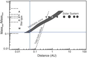
Planets can be tidally locked to their host stars as well. This is a gravitational effect and depends on the mass of the star and the planet’s distance to the star. Over time, the rotation (spin) of the planet is gravitationally synchronized with the orbit. Figure 8 below summarizes where the “tidal lock radius” line (to the left of this line a planet is tidally locked) for stars by their spectral type and the distance that a planet is from the star. Our solar system is shown for comparison. Mercury is shown to the left of the tidal lock radius line, and Mercury is in a 3:2 orbital resonance with the Sun (because it also experiences gravitational pulls from Venus, Mercury is not in a 1:1 orbital resonance, which is the case for tidal locking).

Concept Check: Tidally locked?
Using Figure 8, determine if the exoplanet Proxima b tidally locked around its host star Proxima Centauri.
To answer this using Figure 8, we need the mass of Proxima Centauri and the distance that Proxima b is from this star; these are (source):
MassProxCen = 0.12 MSun
aProxb = 0.0486 AU
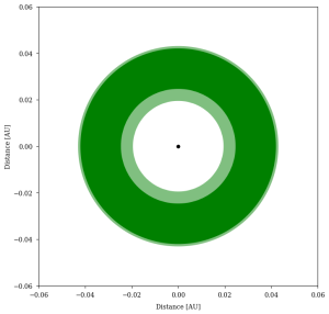
Finding the intersection of these points on Figure 8, the exoplanet is close enough to be tidally locked. This figure also shows that Proxima b falls into the habitable zone around its star. The marked figure is shown below for clarity.
Key Concepts and Summary
Each of the observational detection methods for exoplanets is sensitive to a different range of masses and orbital separations between the host star and planet. In general, larger or more massive exoplanets around the nearest stars present the largest — and therefore most easily detectable — signals. Over the past decades, significant effort has gone into reducing instrumental errors and improving observing strategies with the goal of pressing measurement precision down to Earth-detecting sensitivities. The ensemble of exoplanets and exoplanet architectures reveal some differences from the solar system, however, there are still biases that prevent us from obtaining a full view of planetary systems around other stars. In the TRAPPIST-1 system, seven orbiting planets have been detected. These TRAPPIST-1 planets orbit close to the low mass host star and appear to be terrestrial, or rocky worlds.
Review Questions
Summary Questions
Exercises
- Assessing the habitability of an exoplanet. Choose an exoplanet that you are interested in learning more about, especially the possibility of it hosting life. Begin by hypothesizing whether or not you think the exoplanet is habitable. Go through the four factors (density, surface gravity, habitable zone estimation, and tidal locking) in the Assessing Exoplanetary Habitability section above and discuss whether the evidence you found supports the hypothesis.
