20 Exoplanets: Early History & Direct Imaging and Doppler Detection Methods
Perhaps nothing captures the imagination more fully than envisioning life on another planet. What was still in the realm of science fiction just a few decades ago, especially through television shows like Star Trek, is now commonplace: as of 2024, more than 5,000 exoplanets -- planets orbiting a star other than our Sun -- have been discovered. Their detection and study has brought the search for life in the universe to a new level. Exoplanets can be categorized as rocky or gaseous, and their atmospheres can be searched for biosignatures. Unlocking more clues from exoplanets will narrow down the possibilities for habitable worlds in our galaxy.
Learning Objectives
By the end of this chapter, you will be able to:
- Describe the challenges and progress in taking direct pictures of exoplanets
- Explain the center-of-mass of a solar system and star “wobbling” that enables detection
- Describe how spectra can be used to detect exoplanets (the Doppler Technique) and how the minimum mass of an exoplanet can be found
- Summarize the types of planets (sizes, masses, orbital periods) that can be detected with imaging and radial velocity ("Doppler") data.
Early History
There are several techniques for discovering exoplanets. The first exoplanets were detected by the gravitational effect that they exerted on their host stars. More recent techniques have been able to image the planets. Each method is sensitive to specific types of exoplanets, and when we piece the information together, we can begin to understand the diversity of exoplanets. Humans have long wondered whether other solar systems with planets like our own Earth might exist among the billions of stars in our galaxy, and this moment will go down as the time when we figured this out.
The first failures and successes
The discovery of worlds around other stars has a long history with many false starts. In the 1960s, Peter van de Kamp interpreted a small wobble in the position of Barnard's star as an exoplanet. Observations by other astronomers contradicted that result, although van de Kamp never admitted that his claim was in error. In 1991, Lyne and Bailes reported in the prestigious Nature journal the discovery of a planet orbiting the pulsar star PSR 1829-10. They had measured frequency of pulse arrival times and used the Doppler effect to infer the presence of a planet, but later realized that they had not properly accounted for the velocity of the Earth around the Sun. When Lyne retracted the result at a meeting of the American Astronomical Society in January 1992, he received a standing ovation for his scientific integrity and courage.
There were also a few signals that were initially published with alternative interpretations that later turned out to be exoplanets. In 1988, Campbell, Walker and Yang observed a periodic radial velocity signal in the red giant star, Gamma Cephei. They tentatively interpreted this as photospheric variability in the star, but additional data by Hatzes and colleagues in 2002 confirmed that this was indeed an orbiting exoplanet. Another example occurred in 1989 when Latham and colleagues published the discovery of a companion to the star HD 114762; the team cautiously interpreted this as a possible brown dwarf. However, by 2012, this object was reclassified as a massive exoplanet.
The first confirmed exoplanets were very peculiar. Aleksander Wolszczan and Dale Frail measured periodic variations in the frequency of pulse arrival times to detect two small planets orbiting the pulsar neutron star, PSR 1257+12 in 1992. In 1994, they found one more planet in this system. These discoveries were puzzling because this planetary system should not have survived the supernova explosion of the host star before it evolved to become a spinning neutron star. The planets likely formed in a debris disk around the pulsar. In retrospect, perhaps that discovery should have told us that planet formation was a ubiquitous process. If planets can form around an exploding supernova, then we should have expected that exoplanets were common.
In 1952, astronomer Otto Struve made the remarkable assertion that if a Jupiter-like planet resided very close to its host star, that the gravitational tug of the planet on the star would produce radial velocity variations that might be detected in the stellar spectra with high enough precision measurements.
Twentieth-century astronomers worked to improve the precision of their techniques, and in 1995, the first exoplanet was finally discovered around a sun-like star. Most astronomers consider the dawn of exoplanets to be November 1995 when Michel Mayor and Didier Queloz discovered a gas giant planet orbiting the sun-like star 51 Pegasi at the Observatoire de Haute-Provence using the Doppler technique. The interpretation of this radial velocity signal as an exoplanet remained controversial for a few years but is no longer questioned. 51 Peg b was the first confirmed detection of an exoplanet around a main sequence star, and the 2019 Nobel Prize was awarded to Mayor and Queloz.
Direct Imaging
Just take a picture!
Seeing is believing, so it would be ideal if we could simply point a telescope at a star and take a picture of the orbiting planets. This method is called direct imaging, and the biggest challenge is separating the reflected light of the planet from the light of the star. The problem is that the planet is typically a billion times fainter and lost in the glare of the star.
Coronagraphs
One way to block out the light from a star so that some of the faint planets orbiting the star can come into view is to use an instrument called a coronagraph. Conceptually, this is similar to trying to see a faint object (like a tennis ball, coming over the net) that is lost in the glare of the Sun. If you use your hand to cover the Sun, you can now see the tennis ball. If you were lucky enough to be in the path of totality under clear skies during the solar eclipse of 2017, then you had the perfect demonstration of how a coronagraph works. In this case, the moon acted as a coronagraph, allowing people to see stars close to the Sun in the "day" sky.
The video below is an animation showing how a coronagraph works. Before the light from the star can reach the detector, the coronagraph is used to artificially block out the starlight so that the image captured has most of this glare removed, as seen at the end of the animation when the exoplanet is revealed.
Using a Coronograph to see the planets
Direct Imaging. What happens to the brightness of the orbiting planet when a coronograph is used to block light from the host star?
Animation source: https://exoplanets.nasa.gov/
Coronagraphs were developed in the 1930s by French astronomer Bernard Lyot, who was interested in studying the Sun's corona. Light from the Sun's photosphere completely blocks out the light from the corona, except during a total solar eclipse, so this was a technique that made studying the outer layers of the Sun possible. After exoplanet detections began ramping up in the early 2000s, coronagraphs began being used to take pictures of exoplanets. Coronagraphs still pose extreme challenges and only planets that are sufficiently far from their host stars can be revealed this way.
At the Keck telescope in Hawaii, astronomers used the adaptive optics (AO) system with a coronagraph to detect four planets orbiting the star HR 8799. This star was selected as a good target because it is relatively close (about 40 parsecs from the Sun) and because the star is young (a mere 30 million years) so that any planets would also be young and luminous. Exoplanets are named with lower case letters beginning with "b" in the order that they are discovered. In the image below, planets b, c, and d were found in 2008 and planet e was discovered a few years later. It is challenging to find planets close to the star where the coronagraphic suppression of light is more difficult.
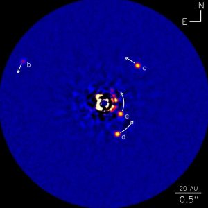
Once the light from the planet's host star has been suppressed with a coronagraph, more information about the properties can be gleaned using other methods. Spectroscopy of the four planets around HR 8799 has been carried out using the Project 1640 instrument on the Palomar telescope and shows variable amounts of absorption from water, carbon monoxide, carbon dioxide, and methane.
The search for exoplanets using coronagraphs is an exciting technique, and impressive technological advances in this field are permitting the detection of smaller planets located at smaller inner working angles (i.e., closer to the star). The James Webb Space Telescope has coronagraphs built into several of its infrared cameras, such as NIRcam and MIRI. In 2023, JWST took its first direct images of the exoplanet HIP 65426 b. The goal for the next 20 years is to develop space-based coronagraphs on large telescopes to image Earth-like planets around nearby stars and to obtain spectra to search for signatures of life.
Star Shades
Another way to block out starlight to enhance planets is to use a star shade. While coronagraphs are built into the telescope's optics, star shades are completely separate from the spacecraft carrying the telescope. The figure below shows the basic layout of a starshade system: the starshade would fly in formation with the spacecraft at a nearly fixed distance in front. And this distance is not tiny -- the starshade needs to be located somewhere between 20,000 to 40,000 km ahead of the spacecraft, depending on the size of the spacecraft.

The distances need to be extremely precise, down to 1 meter (3.2 feet), to avoid having unnecessary light from the star leak through and contaminate the image. This is a technological challenge but engineers at NASA's Jet Propulsion Lab have carried out computer simulations that show this is feasible to do. The upcoming Nancy Grace Roman Space Telescope infrared mission will have a coronagraph on board and there is discussion of adding a starshade as well. The next generation of telescopes to image planets, such as NASA's Habitable Worlds Observatory (HWO), will include a coronagraph and a starshade.
Adaptive Optics
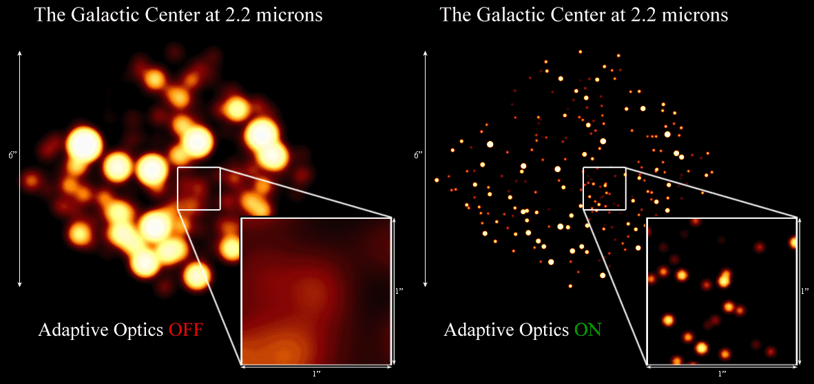
To obtain direct images of exoplanets around nearby stars with ground based telescopes, a technique called adaptive optics (AO) has been developed to correct for the atmospheric twinkling of starlight. AO combines optics, electrical engineering, and computers to correct for atmospheric distortion. In cases where there is more than one star in the field of view of the telescope, light from one of the nearby bright non-science stars is picked off with a mirror and sent to the AO system. If a bright star is not nearby, then a laser can be used to simulate a star on the sky. Hundreds of actuators on a deformable mirror in the AO system are moved around at high speed (thousands of Hertz) until the image of the star is concentrated into the smallest possible point of light. This counteracts the atmospheric distortion for all stars in the field of view, including the science star of interest.
Direct imaging is the only method for finding exoplanets where the planet is directly seen. In the other methods, we must instead infer the presence of exoplanets by how they affect the star they are orbiting, either the star's motion or its brightness. These methods rely upon indirect detection.
The Doppler Technique
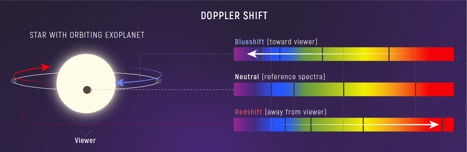
The Doppler technique (also called the radial velocity technique) was the first method to successfully detect exoplanets orbiting Sun-like stars. This technique measures the velocity of stars over time. All stars are traveling in orbits around the center of our Milky Way galaxy. For example, the Sun takes about 220 Myr to complete one loop around the galaxy. As the Sun travels around the galaxy, some stars appear to be moving toward us while others are moving away.
After subtracting the constant galactic velocity for a given star, a small remaining periodic motion in the velocity of a star (a "residual" velocity) can reveal that the star is being tugged around a common center-of-mass by another body, as shown in Figure 5 below. These residual velocities can be modeled to determine whether the orbiting object is a planet. With the Doppler technique, the planet is never observed (making this an "indirect" detection method). Instead, the time-varying velocity of the host star is modeled to infer the presence of an unseen planet. All stars have some nearly constant radial velocity; stars that exhibit a residual periodicity in their radial velocities have a gravitationally bound companion.
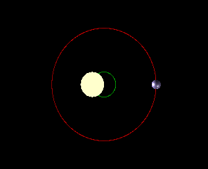
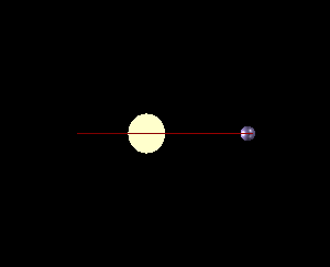
The Center-of-Mass of Solar Systems
The Sun is generally assumed to be the center of our solar system, with the planets, asteroids and comets all orbiting around it. This is almost true but there is a gravitational pull on the Sun from the planets, especially the massive planets. This tug on the Sun causes it to "wobble" around, moving in small loops. This looping pattern repeats but the center stays fixed and is called the center-of-mass. The center-of-mass is the point around which both the star and all planets revolve. This is shown in Figure 5a and 5b (left and right), where for simplicity, there is only one planet orbiting the star.
The Doppler Effect and Radial Velocity
How can this wobble of a star be used to detect exoplanets? The answer brings us back to spectroscopy. Specifically, the Doppler effect, which gives this technique its name. By taking a spectrum of a star, we can determine its temperature, chemical composition and motion. The motion we can find is called the radial velocity and is specifically the motion either directly toward or directly away from us. Think of drawing a radius between the instrument (a spectrograph) and the star -- it is motion along this radial line we can determine. When a star (or any object emitting waves) is moving away from us, its spectral lines are shifted toward smaller wavelengths; this is called a blueshift. When the star is moving away from us, the spectrum shifts toward longer wavelengths, and this is called redshift. Figure 6 shows how this looks for the absorption lines in the spectrum of a star: the middle panel shows the lines if the star has no radial motion; in the top panel, the star is moving away from us and its lines are moved toward the red end of the spectrum; and in the bottom panel the star is moving away from us and its lines are moved toward the blue end of the spectrum.

If we observe a star long enough and find that its spectral lines are shifting back and forth, then the presence of another object (in this case, a planet) can be inferred. Keep in mind that the spectral lines we observe are for the star and not the planet; the planet's reflected light is far too faint to have its spectrum recorded. This can be seen in the animation below (Figure 7), where the spectral lines are for the star.
In reality, high-resolution spectra are needed to find the wavelength shifts to the precision needed to determine properties of an exoplanet. A segment from an extracted high-resolution spectrum around the deep pair of sodium absorption lines is shown in the animation (Figure 8) below, where each shift of the spectrum simulates a different velocity shift. By measuring the periodic shift of the wavelengths for these lines ([latex]\Delta \lambda[/latex]) relative to the rest wavelength ([latex]\lambda_0[/latex], indicated by the red vertical lines for sodium), the velocity of the star over time can be calculated.

The animation above is an extreme exaggeration (for the purpose of illustration) of the reflex Doppler shift that would occur from orbiting exoplanets. The spectral absorption lines in the animation above are between 5-20 pixels in width. A spectral line shift of just one pixel on a detector corresponds to a radial velocity change of about 1000 m/s. The amplitude of Doppler shifts caused by exoplanets would be invisible to the eye on the scale shown above.
To determine the radial velocity of a star from its spectrum, you only need to measure how far the wavelengths of the absorption lines have shifted due to the motion toward or away from us. This shift in wavelength, [latex]\Delta \lambda[/latex], is related to the radial velocity, [latex]v_{rad}[/latex], as follows:
[latex]\frac{\Delta \lambda}{\lambda_0} = \frac{v_{rad}}{c}[/latex]
Here, [latex]{\lambda_0}[/latex] is the wavelength of a line if there was no radial motion, meaning the middle panel of Figure 6. We sometimes refer to [latex]{\lambda_0}[/latex] as the rest wavelength or lab wavelength. The constant [latex]c[/latex] is the speed of light.
This same formula will give the reflex radial velocity for a star that is wobbling due to the presence of a planet, as shown in the example below.
Worked Example: Finding the Reflex Radial Velocity
You observe a star and notice that the spectral lines are moving back and forth. You know that the rest wavelength, [latex]{\lambda_0}[/latex], of one of the lines is 656.28 nm and observe over time that it shifts back and forth by 0.00012 nm (a very small shift). What is the reflex radial velocity of this star?
We are given the shift in wavelength: [latex]\Delta \lambda[/latex] = 0.00012 nm and that the rest wavelength is 656.28 nm. In one step, we can find the reflex radial velocity:
[latex]\frac{v_{rad}}{c} = \frac{\Delta \lambda}{\lambda_0}[/latex]
[latex]v_{rad} =c \frac{\Delta \lambda}{\lambda_0}[/latex] = (3.0×10⁸ m/s)×(0.00012 nm)/(656.28 nm) = 54.8 m/s
Notice that the units of [latex]\Delta \lambda[/latex] and [latex]{\lambda_0}[/latex] are the same -- they are both in nanometers. They can be in any units as long as they are the same and thus cancel each other out.
What does this value mean? This is the reflex (or residual) radial velocity -- as the star moves in its small loop, the radial velocity varies and 54.8 m/s is the maximum value it reaches. The value will reach a maximum speed of 54.8 m/s and a minimum speed of -54.8 m/s. Figure 10 below shows this idea, where in that case E is the maximum and A is the minimum value for the radial velocity.
Our ability to detect smaller planets is limited by the precision with which we can measure the shifts of spectral lines. Jupiter induces a radial velocity in the Sun of about 12 m/s with a periodicity of about 12 years. To detect Jupiter, we would need to measure a 12-year back-and-forth shift in the spectral lines of just 0.01 pixel. (The raw data collected by a spectrograph records data as pixels; the pixels are converted to wavelengths during processing.) This requires that we control the stability of our instrument to much better than this precision and maintain the control over at least 12 years. Impressively, this is the state of the art: astronomers can measure wavelength shifts to the level of 0.001 pixel (1 m/s) with decades-long stability. However, detecting the stellar reflex velocity from a planet like the Earth is a much greater challenge. The Earth induces a velocity of about 10 cm/s in the Sun. This corresponds to a one-year back-and-forth shift of 0.0001 pixel. New instruments are now being developed to try to find other examples of Earth-like planets that might harbor life.
Mass and Inclination of a Planetary System
Kepler's Third Law relates the orbital period of a planet around a star to the planet's average distance from the star: [latex]P^2=a^3[/latex], where [latex]P[/latex] is how long it takes the planet to make one orbit around the star and [latex]a[/latex] is the semi-major axis of the orbit (or the average distance of the planet from its star). This handy version requires that [latex]P[/latex] be given in years and [latex]a[/latex] given in astronomical units (AU). After formulating the Law of Gravitation, Newton generalized this law to include the masses of the two orbiting objects (for a review, see Newton's version of Kepler's Third Law):
[latex](M_{1}+M_{2})P^2 = a^3[/latex]
This means that if we know [latex]P[/latex] and [latex]a[/latex], we can get the total mass of the planetary system. The mass of the star can be estimated based on its spectral type, so this means we can find the mass of the exoplanet! But the full mass of the exoplanet cannot always be determined -- it depends on the orientation of the star system.
Looking carefully at Figure 5 again, notice that we are essentially viewing the star system edge-on, meaning that all of the star's movement is toward/away from us and along our line-of-sight. But what if the planetary system was tilted along our line of sight? Let's imagine the extreme case where we are seeing viewing the system face-on, as in the right panel in Figure 9.

In the case of a face-on orientation of the planetary system, as shown on the right in Figure 9, none of the stars motion is along out line of sight so the Doppler technique will not yield any information. In reality, planetary systems can have any orientation along our line of sight. The orientation of a planetary system is characterized by a parameter $i$, which stands for inclination. For the edge-on case, $i$ = 90° and for the face-on case, $i$ = 0°. For a system that has an inclination that is less than 90°, the exact mass cannot be determined but the minimum mass that the planet could have is found. The minimum mass depends on $\sin i$, and a full quantitative description of how to find this minimum mass is given in the box below.
Detecting planets from velocities
To detect a planet with the Doppler technique, many spectra must be obtained that span the complete orbital period of the star-planet system. Of course, astronomers don't know the orbital period in advance, so in practice, they take as many spectra as possible and then use mathematical and statistical methods to search for repeating changes in the radial velocity.
Figure 10 depicts the orbit of a star as a dashed circular path that is viewed edge-on by an observer to the right. The velocity of the star is constant in this figure, however the projected radial velocity along our line of sight is changing. At point A, the star moves toward the observer and the spectrum of the star is blue-shifted (the measured wavelengths are shorter). At point E, the star moves away from the observer and the spectrum of the star is red-shifted (the measured wavelengths are shifted to longer, redder wavelengths). At point C, there is no radial velocity - all of the motion is tangential to our line of sight. At points B and D, only the projected radial component of the velocity (velocity times the sine of the orbital inclination) can be measured in the stellar spectrum.

The radial velocity data for the star can be used to find the orbital parameters -- and determine the minimum mass -- of the planet. Details are given in the box below.
Want to know more: Finding exoplanet masses from velocity data
From the radial velocity curve of the star, the orbital period of the planet can be found (it is the same as the observed period for the star's wobble) along with the amplitude of the radial velocity for the star. The semi-amplitude, which is half of the full amplitude, is denoted as K and is shown in Figure 11 below.

The orbital parameters can then be used to calculate the semi-major axis and the mass of the planet times the orbital inclination using Newtonian physics.
[latex]K = \frac{1}{\sqrt{1-e^2}} \left(\frac{2 \pi G}{P}\right)^{1/3} \frac{m_{p} \sin(i)}{\left(M_{*}+m_{p}\right)^{2/3}}[/latex]
where
[latex]m_{p}[/latex] is the mass of the exoplanet,
[latex]M_{*}[/latex] is the mass of the star,
[latex]P[/latex] is the orbital period,
[latex]e[/latex] is the eccentricity of the exoplanet's orbit and
[latex]i[/latex] is the inclination of the orbit.
This can be rearranged to give the formula for the minimum mass of the exoplanet:
[latex]m_{p}\sin i = K \sqrt{1-e^2} \left(\frac{P}{2 \pi G}\right)^\frac{1}{3} \left(M_{*}+m_{p}\right)^\frac{2}{3}[/latex]
Statistical probability for [latex]\sin(i)[/latex]
For randomly oriented inclinations, the probability of drawing a particular [latex]\sin(i)[/latex] is not uniform. Instead, the probability of observing an orbit with an inclination $\Delta i$ between $i_{1}$ and $i_{2}$ scales as the difference between the cosine of those angles:
[latex]\mathcal{P}=|\cos i_{1} - \cos i_{2}|[/latex]
So, there is an 86% probability that the inclination of a random orbit is between 90° and 30°. For these typical orbits, the true mass of the planet would be within a factor of two of the measured [latex]m_{p} \sin i[/latex]. Conversely, there is only a 14% probability that an orbital inclination is between 30° and 0° (yielding a true mass more than twice [latex]m_{p} \sin i[/latex]).
Real-world examples
In 1995, Michel Mayor and Didier Queloz discovered the first exoplanet around a main sequence star using the Doppler technique. The planet that they discovered has a mass similar to Jupiter's and orbits the star 51 Pegasi once every 4.23 days. The data from their 1995 discovery paper are shown in Figure 12 below. Because the signal repeats, the velocities can be folded so that the orbital periods repeat. This "phase-folded" data is a helpful way to display relatively short periodic signals and clearly demonstrates that the signal is repeating in a predictable way.
In the data from the Mayor & Queloz 1995 paper, you can see that from September to November in 1994, the radial velocities for 51 Pegasi were changing. This perplexed Didier Queloz, who was a graduate student working with Professor Mayor. To better understand the velocity variations, he began taking more data. Mayor and Queloz developed a mathematical model (shown as the solid line) that fits the velocity changes of the star and also describes Keplerian orbital motion. It is quite an empowering feeling to develop a model like this and to then watch the future velocities of the star follow your predictions.

Queloz and Mayor could not quite believe what they were seeing. A Jupiter-mass planet in a 4-day orbit was very different from any of the planets in our solar system. In their paper, they discuss the alternative interpretations such as stellar pulsations and effectively rule them out. They conclude that the most likely interpretation is an orbiting planetary mass companion. Massive exoplanets that are orbiting very close to their host star are called hot Jupiters. 51 Peg b is considered the poster child for hot Jupiters.
Because they derive the minimum mass, they note that the true mass may be larger than one Jupiter mass. Some skeptics believed that Mayor and Queloz had simply detected a stellar binary system that was oriented nearly face-on, which is a totally reasonable scenario to consider. However, an inclination of less than 1° is required to pump the minimum mass up to the stellar mass regime of 70 Jupiter masses. It can be rigorously shown that probabilistically there is only 1 chance in 10,000 that they would have observed such a low inclination orbit.
Want to know more: the first few exoplanet discoveries
Mayor and Queloz's discovery of an exoplanet in such a short orbital period was a game-changer. A team of astronomers at San Francisco State University were also trying to find exoplanets using the Doppler technique. They had a backlog of data because they were collecting about 50 spectra per night, but it took 24 hours to analyze a single spectrum on the slower computers of the day. Spurred on by the discovery of 51 Peg b, Sun Microsystems made a donation to the SFSU team and they quickly crunched through their observations, discovering Jupiter-like planets around 70 Virginis and 47 Ursa Majoris in their sample of 120 stars. The second of these, 47 UMa b, was very much like 51 Peg b - a Jupiter-mass planet in an orbit of just a few days.
However, the data for 70 Vir b (shown below) told a different story. Instead of the sinusoidal velocity variation seen with 51 Peg b, this planet has a more peaked velocity variation revealing an orbit with eccentricity of 0.4. The planet mass (6.6 times the mass of Jupiter) is also much larger, producing greater velocity variations in 70 Virginis. To the skeptics, the discovery of yet another massive planet was further support for the idea that nearly face-on binary star systems were being discovered rather than exoplanets. The fact that this object was in an eccentric orbit added to the doubts - planets in our solar system are in nearly circular orbits. Surely the rest of the cosmos would be like us?

Practice with the radial velocity simulator
There are a lot of concepts to understand with the Doppler technique. First, we use the spectrum of the star to measure wavelength shifts that correspond to changes in the velocity of the star. Second, we see only the projected radial component of the stellar velocity (this leads to a sinusoidal variation in the signal). Third, we don't know the inclination of the orbit - this tilt of the orbit means that the sinusoidal signal will be largest when viewed edge-on (90° inclination) and smaller as the inclination tilts toward face-on. This means that we only measure the minimum mass ($m_{p}\sini$) with the Doppler method.
Let's get some practice with the Nebraska Astronomy Applet Project (NAAP) Radial Velocity Simulator to help develop your intuition and understanding of the Doppler method. Simulated radial velocities are "phase-folded" in the upper right hand plot. The radial velocities are obtained as a function of time, but if you repeat observations over more than one orbital period, the data can be folded so that all of the peaks and troughs of the curve line up. This is routinely done by astronomers to build evidence for repeating signals.
The default shows a star with the mass of the Sun being orbited by one Jupiter-mass planet with a perfectly circular (eccentricity is zero) orbit; the system is completely edge-on, with an inclination of 90°. To change values, you can either enter them in the box (be sure to hit the return key) or use the sliders. What happens to the radial velocity as you lower the inclination? (Recall that a face-on system has an inclination of 0°.)
Key Concepts and Summary
In 1995, a planet was detected orbiting the sunlike star 51 Pegasi, launching the new field of "exoplanets" in astronomy. There are several different ways to detect exoplanets. Here we reviewed two methods for detecting exoplanets: direct imaging, where the light from the host star is suppressed so that the planet can be observed and the "Doppler" method, which detects the gravitational tug from an unseen planet that changes the radial velocity of the host star. Each of these observational methods is sensitive to different masses and orbital distances of planets.
Review Questions
Summary Questions
- What is the main challenge faced in taking pictures (direct imaging) of exoplanets?
- What is meant by the center of mass of a solar system? Make a sketch to help convey this idea.
- How can the absorption spectrum of a star be used to show that the star has exoplanets orbiting around it?
- How can the shift in spectral lines for a star with a planet be used to find the radial velocity of the star?
- How can Newton's version of Kepler's Third Law be used to find the mass of a planet?
- Why can only the minimum mass be found? In other words, what is needed to find the full mass?
Exercises
- Consider the two methods for detecting exoplanets discussed in this chapter and make a chart listing the advantages of each method and what type of exoplanet it is best at finding.
- RV simulator activities
A planet beyond our Solar System.
