Week 2: Evidence of Evolution: Population Genetics
Objectives
- Describe evidence of evolution that is based on microevolution and population genetics.
- Define and use the terminology of population genetics correctly.
- Use the equations of the Hardy-Weinberg equilibrium to calculate allele and genotype frequencies.
- Graph allele frequencies using Microsoft Excel and identify changes in allele frequencies.
- Draw graphs and explain three types of selection.
This lab begins with a brief overview of the Hardy-Weinberg Theorem and then includes two activities in which you apply the theorem. In the final section of the lab, you will consider what type of selection was at work in Activity 2.
I. Hardy-Weinberg Theorem
Direct evidence of a population that is evolving is a change in allele frequencies. The Hardy-Weinberg Theorem is one way to determine whether allele or genotype frequencies are changing from generation to generation. It states that under the conditions listed below, alleles and genotype frequencies do not change from generation to generation. As you know, most of the conditions (assumptions) are not met in real populations, and therefore, populations evolve.
Changes in allele frequencies can be calculated based on the following equations:
p + q = 1
p = frequency of dominant alleles in a population
q = frequency of recessive alleles in a population
Squaring both sides (p + q)2 = 12 will yield:
p2 + 2pq + q2 = 1
p2 = frequency of homozygous dominant genotypes (individuals) in a population
q2 = frequency of homozygous recessive genotypes (individuals) in a population
2pq = frequency of heterozygous genotypes (individuals) in a population
The conditions (assumptions) of the Hardy-Weinberg Equilibrium are:
- No mutations
- Random mating
- No natural selection
- Extremely large population size
- No gene flow
- No genetic drift
Key Terms
| Term | Definition |
| Microevolution | Microevolution is a change in allele frequencies in a population over generations |
| Alleles | Alternative forms of a gene, or variations of a gene |
| Natural selection | Differential survival and reproduction of individuals in a population of a particular species |
| Gene flow | The movement of alleles among populations due to immigration and/or emigration |
| Speciation | The origin of new species |
| Mutation | Changes in the nucleotide sequence of DNA |
| Genetic drift | Fluctuations in allele frequencies from one generation to the next that are not based on selection |
| Bottleneck effect | Constriction of the gene pool due to natural disasters (this is one example of genetic drift) |
| Founder effect | Constriction of the gene pool when a few individuals become isolated from a larger population (another example of genetic drift) |
| Directional selection | Favors individuals at one end of the phenotypic range |
| Stabilizing selection | Favors intermediate variants and acts against extreme phenotypes at either end of the phenotypic range |
| Disruptive selection | Favors individuals at both extremes of the phenotypic range and acts against intermediate variants |
| Homozygous | Having two identical alleles at a particular locus |
| Heterozygous | Having two different alleles at a particular locus |
| Dominant | An allele that suppresses the expression of a recessive allele in a heterozygote |
| Recessive | An allele whose expression is suppressed if a dominant allele is present (as in heterozygotes), but expressed in the homozygous state |
Pre-lab Activity
View the following videos on the effect of natural selection before coming to lab:
Activity 1: Selection on Prey by a Predator, White and Black Alleles
In this activity, you will apply the Hardy-Weinberg Theorem to determine how allele frequencies change from generation to generation of a prey species being hunted by a predator.
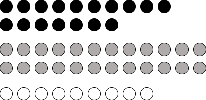
1. Use the figure below to simulate the selection of the prey by the predator. These circles represent the prey species, and their colors represent variations (such as the ability to hide or to run fast) that may help them avoid being hunted and eaten by a predator. There are two alleles for the color gene, white (p) and black (q). The gray individuals are heterozygous.
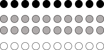
2. Now, you will act as the predator and “hunt” the circles (prey) by drawing an X through 3 white circles, 2 gray circles, and 1 black circle according to the following directions:
a. Set 30 seconds on the timer on your phone, and then start the countdown and your hunt.
b. Place your first X through the white and count to 10 before drawing the next X (about 3 seconds). If you have crossed out 3 white, 2 gray, and 1 black and you still have time left on the clock, repeat the same pattern until your 30 seconds is up. But remember to leave a little time (3 seconds or so) between each “attack” (represented by drawing an X), or you will run out of prey before the 30 seconds is up.
3. The number of each color that you hunt (3 white, 2 gray, 1 black) represents the advantage that each prey variation has. You can find and eat more white than black because white is less well adapted than the black. Based on the instructions given here, which color do you think is the best adapted to avoid predation? Write a hypothesis about what will happen to the frequency of each allele over time.
4. When the 30-second hunt is over, see how many survivors are left (circles not crossed out are survivors). Use the number of survivors to calculate p and q as shown in the example below. Once you have p and q, you will calculate p2, 2pq, and q2 and use those numbers to predict how many circles of each color there will be in the next generation, as shown in the example below.
Example
Calculations for generation 1
In generation 1, the allele and genotype frequencies are as follows:
CWCW = Homozygous (white)
CWCB = Heterozygous (gray)
CBCB = Homozygous (black)
We will designate the white allele CW as p, and the black allele CB as q. There are 40 individuals in the original population, which means there are 80 alleles total since the individuals are diploid.
10 white circles
20 gray circles
10 black circles
p = [(2 x 10) + 20]/80 = 0.5
p + q = 1, therefore, q = 0.5
If you are not sure why p and q are calculated in this way, please review the videos, reading, or slides for this week before continuing.
Calculations for generation 2
Imagine that the following numbers of individuals in generation 1 survive the hunt.
4 white circles
14 gray circles
8 black circles
These numbers may differ from the numbers that survive your first hunt. The purpose of this example is to show you how to figure out the proportions of colored circles for generation 2.
First, we recalculate new p and q values as below. Remember that the white allele is p and the black allele is q.
p = [(2 x 4) + 14]/52 = 0.423, and q = 1 – 0.423 = 0.577
p2 = (0.423)2 = 0.18 (round to two decimal places)
q2= (0.577)2 = 0.33 (round to two decimal places)
2pq = 2 * 0.423 * 0.577 = 0.49 (round to two decimal places)
And then we construct a new population with 50 individuals using the values of p2, 2pq and q2 calculated above. You will need to round up or down to the nearest whole number if the formula gives you a number such as 16.5.
50 * p2 = 50 x 0.18 = 9, so 9 white circles
50 * q2 = 50 x 0.33 = 17 (round up), so 17 black circles
50 * 2pq = 50 * 0.49 = 24 (round down), so 24 gray circles
5. Now draw generation 2 with the predicted values and do the hunt again. For the example above, we would use 9, 24, and 17 and draw the circles as shown below.
Remember, however, that you should draw circles representing the numbers you calculated from your own hunt rather than these example numbers.
6. Now hunt again, as you did before, and record the number of survivors in your lab report. Then calculate new allele and genotype frequencies.
7. Based on the new allele and genotype frequencies you calculated, construct a new population (generation 3) of 50 individuals.
8. Now hunt again, as you did before, and record the number of survivors in your lab report. Then calculate new allele and genotype frequencies.
9. If you have time, repeat the experiment two more times for a total of five generations. It may be difficult to see a trend and draw any conclusions about your hypothesis with only three generations.
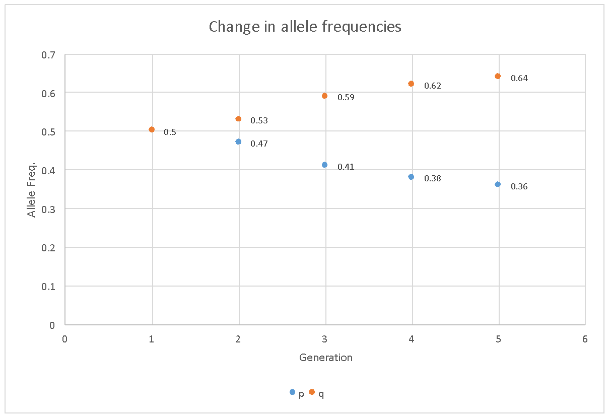
10. Using Microsoft Excel (Kingsborough Community College students have free access to a web version of Excel) or drawing your graph by hand, plot allele frequencies (p and q) and copy and paste your graph into the lab report. Your graph may look similar to the graph in Figure 1 (below). In 3 or 4 sentences in your lab report, describe and interpret your graph. Do the results support your hypothesis?
Activity 2: Selection on Prey by a Predator, White and Red Alleles
In General Biology I you learned about the genetics of the Four O’Clock plant, showing incomplete dominance with:
CRCR plants being red
CRCW plants being pink, and
CWCW plants being white
This genetics of this system of inheritance, called incomplete dominance provide a an easy way to distinguish between homozygous dominants (red) and heterozygotes (pink).
We will use a similar system, except that the genotypes will not represent different colors in the Four O’Clock plant with different colors, but will represent fur color in a prey species that also exhibits incomplete dominance. You will again apply the Hardy-Weinberg Theorem to determine how the allele frequencies change from generation to generation of this species.
1. Secure a tray containing the material that you need as depicted in the photograph below. Work in groups of at least four students per group.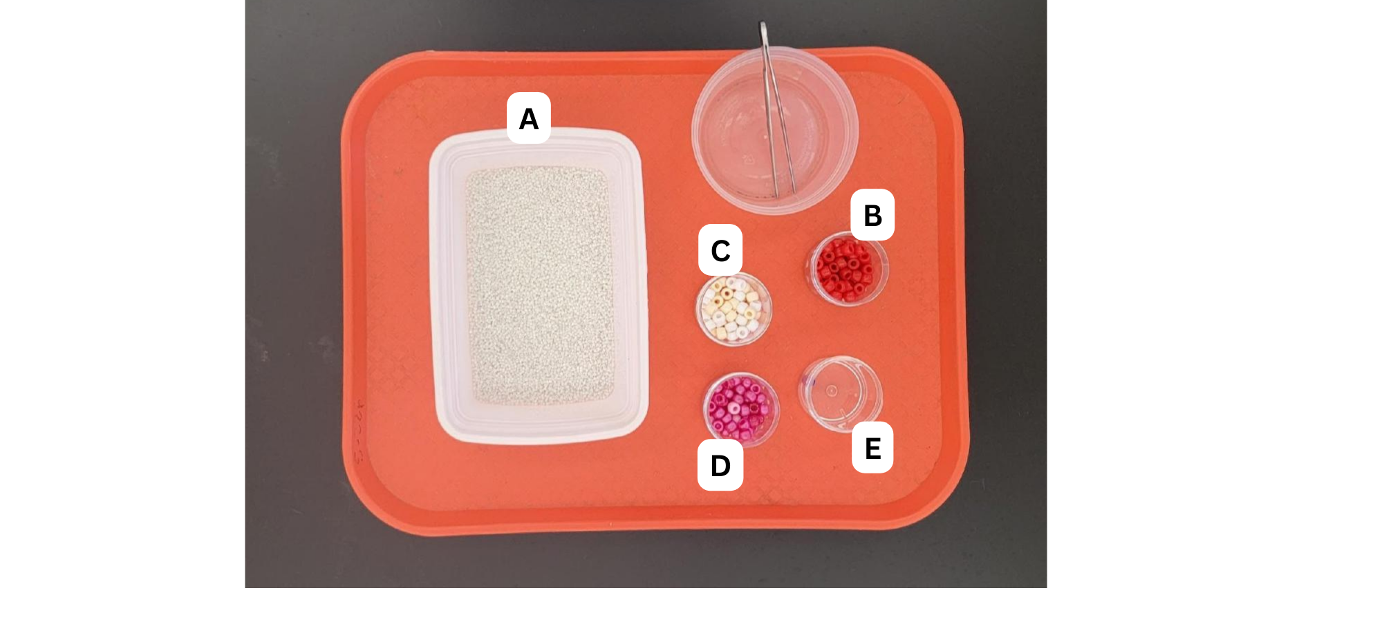
2. Select 10 red beads (B), 20 pink beads (D), and 10 white beads (C). These beads represent the prey species with different colors. The colors represent variations (such as the ability to hide or to run fast) that may help them avoid being hunted and eaten by a predator. There are two alleles for the color gene, red (p, CR) and white (q, CW). The pink individuals are heterozygous (CRCW).
3. Place the 10 red beads (B), 20 pink beads (D), and 10 white beads (C) in the container with small white beads (A). Mix the content. Assume that you are a predator that sees the red beads as not camouflaged, the pink beads as less camouflaged, and the white beads as camouflaged. You will capture an individual prey every 3 seconds for 30 total seconds in the following manner (one bead per every 3 seconds):
a. 3 red beads (take one out, wait 3 seconds, take a second out, wait 3 seconds, take the third one out), then move to the next step
b. 2 pink beads (waiting 3 seconds between each removal)
c. 1 white bead
d. Repeat steps a–c for a total of 30 seconds (one bead per every 3 seconds).
First, write a hypothesis about what will happen to the frequency of each allele (p and q) over time, and then begin the 30-second hunt.
4. When the 30-second hunt is over, see how many survivors are left (represented by beads with different colors). Use the number of survivors to calculate p and q as shown in the example below. Once you have p and q, you will calculate p2, 2pq, and q2 and use those numbers to predict how many beads of each color there will be in the next generation, as shown in the example below.
Example
Calculations for generation 1
In generation 1, the allele and genotype frequencies are as follows:
CRCR = Homozygous dominant (red)
CRCW = Heterozygous (pink)
CWCW = Homozygous recessive (white)
We will designate the white allele CW as q, and the red allele CR as p. There are 40 individuals in the original population, which means there are 80 alleles total, since the individuals are diploid.
10 red individuals
20 pink individuals
10 white individuals
p = [(2 * 10) + 20]/80 = 0.5
p + q = 1, therefore, q = 0.5
If you are not sure why p and q are calculated in this way, please review the videos, reading, or PowerPoint for this week before continuing.
Calculations for generation 2
Imagine that the following numbers of individuals in generation 1 survive the hunt.
4 red individuals
14 pink individuals
8 white individuals
These numbers may differ from the numbers that survive your first hunt. The purpose of this example is to show you how to do the calculations to figure out the proportions of colored beads for generation 2.
First, we recalculate new p and q values (see below). Remember that the white allele is q and the red allele is p.
p = [(2 x 4) + 14]/52 = 0.423, and q = 1 – 0.423 = 0.577
p2 = (0.423)2 = 0.18 (round to two decimal places)
q2= (0.577)2 = 0.33 (round to two decimal places)
2pq = 2 * 0.423 * 0.577 = 0.49 (round to two decimal places)
And then we construct a new population with 50 individuals using the values of p2, 2pq, and q2 calculated above. You will need to round up or down to the nearest whole number if the formula gives you a number such as 16.5.
50 * p2 = 50 * 0.18 = 9, so 9 red plants
50 * q2 = 50 * 0.33 = 17 (round up), so 17 white plants
50 * 2pq = 50 * 0.49 = 24 (round down), so 24 pink plants
6. Once you have determined the composition of the new generation, repeat the hunting and calculations in the same manner at least twice more. After each 30-second hunt, calculate new p and q values and determine the composition of the next generation based on the newly calculated p2, 2pq, and q2 values.
5. Using Microsoft Excel or drawing your graph by hand, plot allele frequencies (p and q). Your graph may look similar to the graph in Figure 2 (below). In 3 or 4 sentences in your lab report, describe and interpret your graph. Do the results support your hypothesis?
II. Types of Selection
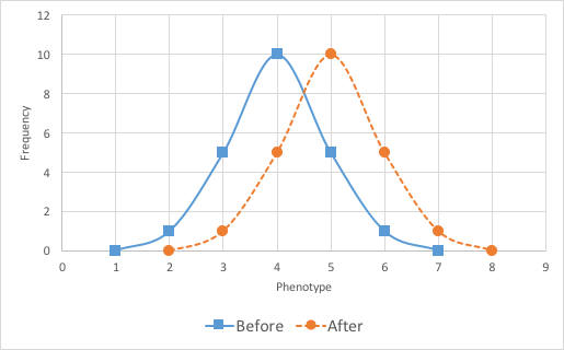
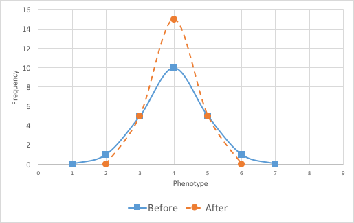
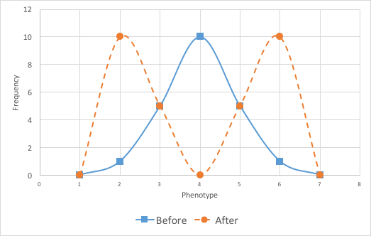
Variation in a population is important for evolution. Natural selection works on individuals’ phenotypes. In general, if there is selection, it may select for or against particular phenotypes. The figures below depict three possible scenarios (Figures 3A–3C). In your lab report, indicate which type of selection was at work in Activity 2.
1. Directional selection: A particular phenotype at an extreme end is being selected for, shifting the resulting population with respect to that particular phenotype to the right (below) or left (also possible).
2. Stabilizing selection: A particular intermediate phenotype is being selected for, resulting in a population with less frequency in extreme phenotypes and more of the intermediate phenotypes.
3. Disruptive selection: Phenotypes at the extremes are being selected for, and those that are intermediate are selected against; resulting in a population with more frequency in extreme phenotypes and less of the intermediate phenotypes.