7.3 Dating Planetary Surfaces: Crater Counting (and Other Methods!)
How do we know the age of the surfaces we see on planets and moons? If a world has a surface (as opposed to being mostly gas and liquid), planetary geologists have developed some techniques for estimating how long ago that surface solidified. From afar, we rely on relative age dating and crater counting to estimate ages of surfaces. If we have physical samples from a planetary body, we can use radiometric dating to get a precise formation age.
Note that the age of these surfaces is not necessarily the age of the planet as a whole. On geologically active objects (including Earth), vast outpourings of molten rock or the erosive effects of water and ice, which we call planet weathering, have erased evidence of earlier epochs and present us with only a relatively young surface for investigation.
7.3.1 Relative Age Dating
Relative dating is the process of determining if one rock or geologic event is older or younger than another, without knowing their specific ages—i.e., how many years ago the object was formed. The principles of relative time are simple, even obvious now, but were not generally accepted by scholars until the scientific revolution of the 17th and 18th centuries. James Hutton realized geologic processes are slow and his ideas on uniformitarianism (i.e., “the present is the key to the past”) provided a basis for interpreting rocks on Earth and other planets using scientific principles.
Relative Dating Principles
Stratigraphy is the study of layered sedimentary rocks. This section discusses principles of relative time used in all of geology, but are especially useful in stratigraphy.
- Principle of Superposition: In an otherwise undisturbed sequence of sedimentary strata, or rock layers, the layers on the bottom are the oldest and layers above them are younger (Figure 7.12).
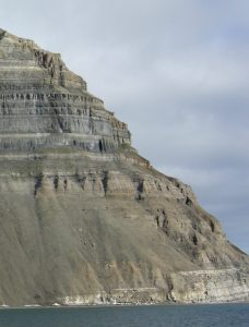
Figure 7.12: Lower strata are older than those lying on top of them. [IsfjordenSuperposition © Mark A. Wilson is licensed under a Public Domain license] - Principle of Original Horizontality: Layers of rocks deposited from above, such as sediments and lava flows, are originally laid down horizontally. The exception to this principle is at the margins of basins, where the strata can slope slightly downward into the basin.
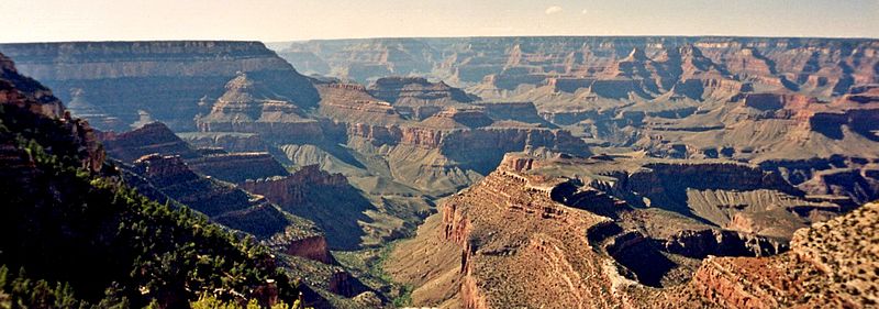
- Principle of Lateral Continuity: Within the depositional basin, strata are continuous in all directions until they thin out at the edge of that basin. Of course, all strata eventually end, either by hitting a geographic barrier, such as a ridge, or when the depositional process extends too far from its source, either a sediment source or a volcano. Strata that are cut by a canyon later remain continuous on either side of the canyon (Figure 7.13).

Figure 7.13: Lateral continuity. [lateral_continuity_Grandview_Point_Grand_Canyon_April_1995 © Ron Clausen is licensed under a CC0 (Creative Commons Zero) license] - Principle of Cross-Cutting Relationships: Deformation events like folds, faults and igneous intrusions that cut across rocks are younger than the rocks they cut across (Figure 7.14).

Figure 7.14: Dark dike cutting across older rocks, the lighter of which is younger than the grey rock. [Multiple_Igneous_Intrusion_Phases_Kosterhavet_Sweden © Thomas Eliasson of Geological Survey of Sweden] - Principle of Inclusions: When one rock formation contains pieces or inclusions of another rock, the included rock is older than the host rock.
- Principle of Fossil Succession: Evolution has produced a succession of unique fossils that correlate to the units of the geologic time scale. Assemblages of fossils contained in strata are unique to the time they lived, and can be used to correlate rocks of the same age across a wide geographic distribution. Assemblages of fossils refers to groups of several unique fossils occurring together (Figure 7.15).
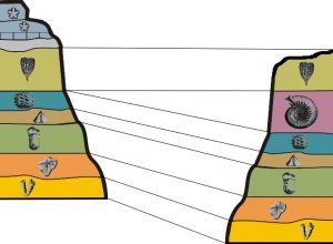
Figure 7.15: Fossil succession showing correlation among strata. [Faunal_sucession © דקי (אני יצרתי) is licensed under a CC BY-SA (Attribution ShareAlike) license]
7.3.2 Counting the Craters
One way to estimate the age of a surface is by counting the number of impact craters. This technique works because the rate at which impacts have occurred in the solar system has been roughly constant for several billion years. Thus, in the absence of forces to eliminate craters, the number of craters is simply proportional to the length of time the surface has been exposed. This technique has been applied successfully to many solid planets and moons (Figure 7.16).
Still, astronomers can use the numbers of craters on different parts of the same world to provide important clues about how regions on that world evolved. On a given planet or moon, the more heavily cratered terrain will generally be older (that is, more time will have elapsed there since something swept the region clean).
Using Crater Counts on the Moon
If a world has had little erosion or internal activity, like the Moon during the past 3 billion years, it is possible to use the number of impact craters on its surface to estimate the age of that surface. By “age” here we mean the time since a major disturbance occurred on that surface (such as the volcanic eruptions that produced the lunar maria).
We cannot directly measure the rate at which craters are being formed on Earth and the Moon, since the average interval between large crater-forming impacts is longer than the entire span of human history. Our best-known example of such a large crater, Meteor Crater in Arizona (Figure 7.17), is about 50,000 years old. However, the cratering rate can be estimated from the number of craters on the lunar maria or calculated from the number of potential “projectiles” (asteroids and comets) present in the solar system today. Both lines of reasoning lead to about the same estimations.
For the Moon, these calculations indicate that a crater 1 kilometer in diameter should be produced about every 200,000 years, a 10-kilometer crater every few million years, and one or two 100-kilometer craters every billion years. If the cratering rate has stayed the same, we can figure out how long it must have taken to make all the craters we see in the lunar maria. Our calculations show that it would have taken several billion years. This result is similar to the age determined for the maria from radioactive dating of returned samples—3.3 to 3.8 billion years old.
The fact that these two calculations agree suggests that astronomers’ original assumption was right: comets and asteroids in approximately their current numbers have been impacting planetary surfaces for billions of years. Calculations carried out for other planets (and their moons) indicate that they also have been subject to about the same number of interplanetary impacts during this time.
We have good reason to believe, however, that earlier than 3.8 billion years ago, the impact rates must have been a great deal higher. This becomes immediately evident when comparing the numbers of craters on the lunar highlands with those on the maria. Typically, there are 10 times more craters on the highlands than on a similar area of maria. Yet the radioactive dating of highland samples showed that they are only a little older than the maria, typically 4.2 billion years rather than 3.8 billion years. If the rate of impacts had been constant throughout the Moon’s history, the highlands would have had to be at least 10 times older. They would thus have had to form 38 billion years ago—long before the universe itself began.
In science, when an assumption leads to an implausible conclusion, we must go back and re-examine that assumption—in this case, the constant impact rate. The contradiction is resolved if the impact rate varied over time, with a much heavier bombardment earlier than 3.8 billion years ago (Figure 7.18). This “heavy bombardment” produced most of the craters we see today in the highlands.
Another way to trace the history of a solid world is to measure the absolute age of individual rocks. Using absolute dating techniques, scientists are able to assign specific time units, in this case years, to mineral grains within a rock. Unlike relative dating, these numerical values are not dependent on comparisons with other rocks, hence the use of the word “absolute” in its name.
After samples were brought back from the Moon by Apollo astronauts, the techniques that had been developed to determine the specific age of rocks on Earth were applied to rock samples from the Moon to establish a geological chronology for the Moon. Furthermore, a few samples of material from the Moon, Mars, and the large asteroid Vesta have fallen to Earth as meteorites and can be examined directly.
Scientists measure the age of rocks using the properties of natural radioactivity. Around the beginning of the twentieth century, physicists began to understand that some atomic nuclei are not stable but can split apart (decay) spontaneously into smaller nuclei. The process of radioactive decay involves the emission of particles such as electrons, or of radiation in the form of gamma rays.
For any one radioactive nucleus, it is not possible to predict when the decay process will happen. Such decay is random in nature, like the throw of dice: as gamblers have found all too often, it is impossible to say just when the dice will come up 7 or 11. But, for a very large number of dice tosses, we can calculate the odds that 7 or 11 will come up. Similarly, if we have a very large number of radioactive atoms of one type (say, uranium), there is a specific time period, called its half-life, during which the chances are fifty-fifty that decay will occur for any of the nuclei.
A particular nucleus may last a shorter or longer time than its half-life, but in a large sample, almost exactly half of the nuclei will have decayed after a time equal to one half-life. Half of the remaining nuclei will have decayed after two half-lives pass, leaving only one half of a half—or one quarter—of the original sample (Figure 7.19).
1/2 gram; after 200 years, 1/4 gram; after 300 years, only 1/8 gram; and so forth. However, the material does not disappear. Instead, the radioactive atoms are replaced with their decay products. Sometimes the radioactive atoms are called parents and the decay products are called daughter elements.
In this way, radioactive elements with half-lives we have determined can provide accurate nuclear clocks. By comparing how much of a radioactive parent element is left in a rock to how much of its daughter products have accumulated, we can learn how long the decay process has been going on and hence how long ago the rock formed. Table 7.1 summarizes the decay reactions used most often to date lunar and terrestrial rocks.
| Parent | Daughter | Half-Life (billions of years) |
|---|---|---|
| Samarium-147 | Neodymium-143 | 106 |
| Rubidium-87 | Strontium-87 | 48.8 |
| Thorium-232 | Lead-208 | 14.0 |
| Uranium-238 | Lead-206 | 4.47 |
| Potassium-40 | Argon-40 | 1.31 |
For Further Exploration
This radioactive decay simulator lets you examine how the number of atoms of a radioactive element decreases over time and see how the ratio of parent to child atoms could be used to figure out the age of the whole set of atoms.
When astronauts first flew to the Moon, one of their most important tasks was to bring back lunar rocks for radioactive age-dating. Until then, astronomers and geologists had no reliable way to measure the age of the lunar surface. Counting craters had let us calculate relative ages (for example, the heavily cratered lunar highlands were older than the dark lava plains), but scientists could not measure the actual age in years. Some thought that the ages were as young as those of Earth’s surface, which has been resurfaced by many geological events. For the Moon’s surface to be so young would imply active geology on our satellite. Only in 1969, when the first Apollo samples were dated, did we learn that the Moon is an ancient, geologically dead world. Using such dating techniques, we have been able to determine the ages of both Earth and the Moon: each was formed about 4.5 billion years ago (although, as we shall see, Earth probably formed earlier than the Moon).
We should also note that the decay of radioactive nuclei generally releases energy in the form of heat. Although the energy from a single nucleus is not very large (in human terms), the enormous numbers of radioactive nuclei in a planet or moon (especially early in its existence) can be a significant source of internal energy for that world. Geologists estimate that about half of Earth’s current internal heat budget comes from the decay of radioactive isotopes in its interior.
Watch the below video which summarizes the use of radiometric dating on Earth rocks.
Text Attributions
This text of this chapter is adapted from:
- Sections 7.3 and 9.3 of OpenStax’s Astronomy 2e (2022) by Andrew Fraknoi, David Morrison, and Sidney Wolff. Licensed under CC BY 4.0. Access full book for free at this link.
- Chapter 7 of An Introduction to Geology (2017) by Chris Johnson, Matthew D. Affolter, Paul Inkenbrandt, and Cam Mosher. Licensed under CC BY-NC-SA 4.0.
Media Attributions
- “Methods of Dating the Earth Part 1: Relative Dating.” YouTube, uploaded by Professor Dave Explains, 16 Oct 2023, https://www.youtube.com/watch?v=F7k1f1TiQ5c&list=PLybg94GvOJ9E5VK94UujanWk45qM8rQuz&index=37.
- “Methods of Dating the Earth Part 2: Absolute Dating (Radiometric Dating).” YouTube, uploaded by Professor Dave Explains, 30 Oct 2023, https://www.youtube.com/watch?v=GwgxCQL2FLc.
