Chapter 1. Psychophysics and Neuroscience.
1.3 Psychophysical Methods
Scientists who study sensation and perception often use psychophysical techniques in their research studies. Psychophysical methods investigate a person’s (psychological) response to a physical stimulus. In other words, how does a physical change in a stimulus affect a person’s perception of it? Psychophysics helps to build a bridge between the physical world and our experience of it. For example, psychophysical methods can help us to determine how loud a sound needs to be before we can hear it or how much sugar we need to add to a cup of coffee to make it noticeably sweeter. Psychophysical methods typically measure people’s sensitivity to sensory stimuli in terms of thresholds. For example, you might describe yourself as someone who is highly sensitive to pain – in other words you have a low threshold for pain. Researchers can measure your threshold for pain with considerable accuracy using psychophysics.
We can measure different types of sensory thresholds, but let’s begin with a common concept in sensation and perception – an absolute threshold. An absolute threshold is the minimum amount of stimulus energy that must be present for a person to detect a stimulus. Another way to think about this is that we can ask how dim can a light be or how soft can a sound be for us to be aware of it The sensitivity of our sensory receptors can be quite amazing. It has been estimated that on a clear night, the most sensitive sensory cells in the back of the eye can detect a candle flame 1.6 miles away (Krisciunas & Carona, 2015) .
Absolute thresholds are generally measured under incredibly controlled conditions in situations that are optimal for sensitivity. There are three common techniques for measuring thresholds.
Psychophysical Methods
- Method of Limits. The experimenter presents stimuli of gradually changing intensity (either increasing or decreasing) until the observer reports a change in perception. If multiple measurements are taken, this method can be time-consuming but provides quite accurate measurements.
- Method of Adjustment. This is very much like the Method of Limits, except the experimenter gives the observer a sliding control to adjust the stimulus intensity until they can just perceive it. This is a much quicker method than the Method of Limits and so may be helpful for participants with limited attention, but it is less accurate.
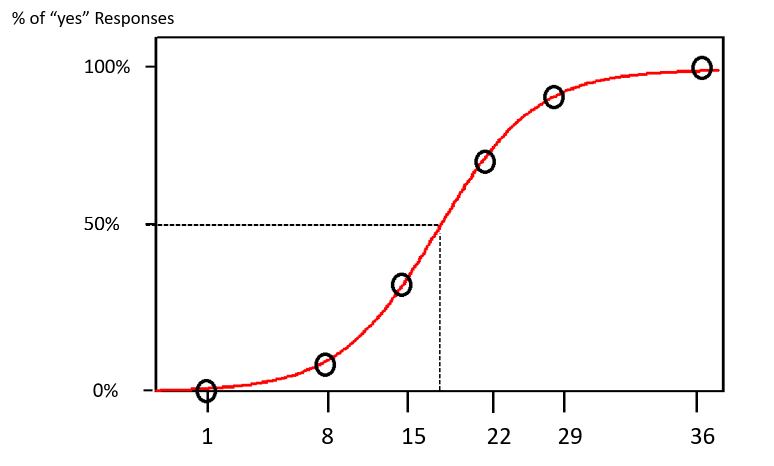
- Method of Constant Stimuli. This is the most reliable, but most time-consuming method. The experimenter presents many stimuli of different intensities in a randomized order and graphs the observer’s responses. The graph is used to calculate the stimulus intensity at which the observer perceives the stimulus 50% of the time.
Let’s take a closer look at these three different methods, with some specific examples to help you to understand what it would be like to be a participant in one of these studies.
Method of Limits
Let’s start with the Method of Limits. Let’s imagine the experimenter wants to measure the absolute threshold for a small circle of light. In other words, how bright does the light need to be in order for us to just be able to see it? As we can see in the left-hand column of Table 1.1, the experimenter first presents a light with very low brightness (1 unit) and asks the participant whether they can see it . They cannot and so they record a “no response” in the table and they then very gradually increase the brightness, one step at a time until the participant says they can see the light (in Table 1.1 below, this occurs when the light reaches 29 units of brightness). The experimenter then stops increasing the brightness and records the response as a “Yes”. This set of steps (from 1 to 29) is called an ascending staircase because the brightness was increasing a little at a time. The threshold on this staircase is estimated to be halfway between the last “no” response (22 units) and the first “yes” response (29 units) i.e., 25.5 units of brightness. This is also called the cross-over point. The ascending trial is then followed by a descending trial. In the descending staircase, the light starts off bright (50 units) and is gradually decreased in intensity until the participant says they can no longer see it (15 units). The cross-over point on this staircase is between the last “yes” response – 22 units and the “no” response (15 units).
It is quite common to have higher thresholds on ascending compared to descending staircases. This is thought to be due to errors of habituation. In other words, we get into a “routine” or a habit of giving the same response. In ascending staircases, the habitual response is to say no, this means we tend to go past the actual threshold before we change to a yes response. The opposite is true for descending trials. One way to try and compensate for these errors is to use multiple and equal numbers of ascending and descending staircases and then calculate the average of the thresholds across all the staircases. In the example below we have two ascending staircases and two descending ones – so we can take the mean of four cross-over points. Experimenters also use different starting points on each staircase type to avoid the participant trying to guess when they should change their response – based on the previous staircases. This helps us to avoid these errors of anticipation. In this example, the first ascending staircase starts on 1 unit of brightness, but the second one (2A) on 8 units.
| Brightness | Ascending staircase (1 A) | Descending staircase (1D) | Ascending staircase (2 A) | Descending staircase (2 D) |
| 50 | Yes | |||
| 43 | Yes | Yes | ||
| 36 | Yes | Yes | ||
| 29 | Yes | Yes | Yes | |
| 22 | No | Yes | Yes | Yes |
| 15 | No | No | No | Yes |
| 8 | No | No | No | |
| 1 | No | |||
| Cross-over point | 25.5 | 18.5 | 18.5 | 11.5 |
Table 1.1. Data collected from a participant using the Method of Limits to calculate the absolute threshold for a small circle of light.
Method of Adjustment.
As in the previous example, the experimenter using the Method of Adjustment can also make multiple measurements and estimate the average across the measures. However, the brightness is adjusted by the participant (not the experimenter) using a sliding scale (like a dimmer switch), so each measurement is taken very quickly. This method is useful when speed is more important than accuracy.
Method of Constant Stimuli
The experimenter presents very many stimuli of different intensities in a random order and asks the observer whether they can see the light for each presentation. Typically more stimuli are presented than in the Method of Limits. The experimenter records the results for each stimulus intensity as a percentage of the times that the participant says that they saw the light. The experimenter will graph the data as in Figure 1.3. Each circle represents multiple trials at that specific intensity. For example, as seen in Figure 1.3, at very high intensities (36 units) a participant will say that they see a light all the time (100%) and at very low intensities (e.g., 1 unit) they will say that they see it none of the time (0%). Therefore, the graph is S-shaped with flat ends, the experimenter would use the graph to find the intensity at which the observer says that they see the light half of the time (50%), which is 17.5 in the example in Figure 1.3. Since there is no predictability to how the stimuli are presented, this method eliminates errors of habituation and anticipation. However, this method is slow and you would need a computer (or good graphing skills) to calculate the threshold (50% mark) for each participant.
Just Noticeable Difference
Sometimes, we are more interested in how much we need to change a stimulus for us to detect that it is slightly different from another very similar stimulus. For example, how much sugar would we need to add to a cup of coffee to notice that it is is sweeter than the previous cup. This is known as the just noticeable difference (JND) or difference threshold. Unlike the absolute threshold, the difference threshold changes depending on stimulus intensity. For example, imagine yourself in a very dark movie theater. If an audience member were to receive a text message on her cell phone which causes her screen to light up, the chances are that many people would notice the change in brightness in the theater. However, if the same thing happened in a brightly lit arena during a basketball game, very few people would notice. The cell phone brightness does not change, but our ability to detect a small change in illumination varies dramatically between the two contexts. If a stimulus is intense, then we need to make a bigger change in intensity in order for us to notice the difference. Ernst Weber proposed this theory of change in difference threshold in the 1830s, and it has become known as Weber’s law. Weber’s law states that the difference threshold is a constant fraction of the original stimulus. The amount of difference we can detect is different across sensory modalities and can be calculated from Weber fractions. For example, the Weber fraction for detecting weight differences is 5% (under optimal testing conditions). This means. that if you have a 100 g weight in each hand, you would need to add about 5g (5% of the original weight) to one weight to tell that it is noticeably heavier than the other. If however, you had 200g in each hand you would need to add twice as much – 10g. Weber’s fraction (5%) is a constant. Weber’s fraction is important in food and drink manufacture, where manufacturers may need to determine how much of a change is needed to make a drink taste just a little saltier (15%), sweeter (17%) or thicker in texture (26%; Camacho et al., 2015).
Magnitude Estimation
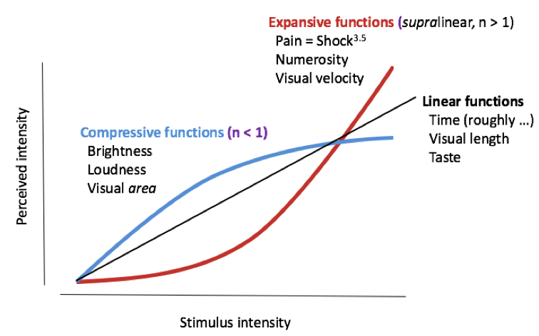
There are times when we want to measure more than a person’s threshold -for example, we might want to know a person’s perception of the intensity of a stimulus- we called this magnitude estimation of perceived intensity. Experimenters can measure perceived intensity at different intensity values to see how accurate we are. For example, we are very accurate in estimating the length of a line once we are given a standard measure to compare it to. On the other hand we tend to overestimate the intensity of an electric shock (response expansion) and underestimate the brightness of a light (response compression). A psychophysical researcher named Stanley Smith Stevens asked people to estimate the magnitude of their sensations for many different kinds of stimuli at different intensities, and then tried to fit lines through the data to predict people’s sensory experiences (Stevens, 1967). What he discovered was that most senses could be described by a power law of the form P ∝Sn
where P is the perceived magnitude, ∝ means “is proportional to”, S is the physical stimulus magnitude, and n is a positive number. If n is greater than 1, then the slope (rate of change of perception) is getting larger as the stimulus gets larger, and sensitivity increases as stimulus intensity increases. A function like this is described as being expansive or supra-linear. If n is less than 1, then the slope decreases as the stimulus gets larger (the function “rolls over”). See Figure 1.4. These sensations are described as being compressive. Stevens’ Power Law is useful for describing a wider range of senses.
Both Stevens’ Power Law and Weber’s Law are only approximately true. They are useful for describing, in broad strokes, how our perception of a stimulus depends on its intensity or size. They are rarely accurate for describing perception of stimuli that are near the absolute detection threshold. Still, they are useful for describing how people are going to react to normal everyday stimuli.
CC LICENSED CONTENT, SHARED PREVIOUSLY
OpenStax, Psychology Chapter 5.1 Sensation and Perception.
Provided by: Rice University.
Download for free at https://cnx.org/contents/Sr8Ev5Og@12.2:K-DZ-03P@12/5-1-Sensation-versus-Perception.
License: Creative Commons Attribution 4.0
Camacho, S., Dop, M., de Graaf, C. and Stieger, M. (2015), Just noticeable differences and Weber fraction of oral thickness perception of model beverages. Journal of Food Science, 80, S1583-S1588. https://doi.org/10.1111/1750-3841.12922
Galanter, E. (1962). Contemporary Psychophysics. In R. Brown, E.Galanter, E. H. Hess, & G. Mandler (Eds.), New directions in psychology. New York, NY: Holt, Rinehart & Winston.
Krisciunas, K., & Carona, D. (2015). At what distance can the human eye detect a candle flame?. https://doi.org/10.48550/arXiv.1507.06270
Kunst-Wilson, W. R., & Zajonc, R. B. (1980). Affective discrimination of stimuli that cannot be recognized. Science, 207, 557–558.
Nelson, M. R. (2008). The hidden persuaders: Then and now. Journal of Advertising, 37(1), 113–126.
Okawa, H., & Sampath, A. P. (2007). Optimization of single-photon response transmission at the rod-to-rod bipolar synapse. Physiology, 22, 279–286.
Radel, R., Sarrazin, P., Legrain, P., & Gobancé, L. (2009). Subliminal priming of motivational orientation in educational settings: Effect on academic performance moderated by mindfulness. Journal of Research in Personality, 43(4), 1–18.
Rensink, R. A. (2004). Visual sensing without seeing. Psychological Science, 15, 27–32.
Stevens, S. S. (1957). On the psychophysical law. Psychological Review 64(3):153—181. PMID 13441853
