20 The Aggregate Model: Aggregate Demand, Long-Run Aggregate Supply, and Short-Run Aggregate Supply
Bettina Berch
Consider this

This chapter brings together a lot of intersecting curves, as we build our model of the economy as a whole, the aggregate model. Do our graphs ever remind you of highways crossings?
In previous sections of this book, we have learned some basic tools of economic analysis and some basic macro concepts: GDP, the price level, full employment, production, growth, money, and more. Now it is time to build our model of the economy as a whole–the aggregate model. Like all models, this macro-model will abstract from real-life details to focus on the underlying dynamics. It will also give us some policy advice–what to do if our economy needs help. The first things we need to understand, however, is that the aggregate model might look like our earlier, simple supply and demand model, but it operates very differently.
The simple supply and demand model versus the aggregate model
As with most economic models, we are still putting a price-type variable on the vertical axis and a quantity-type variable on the horizontal axis.
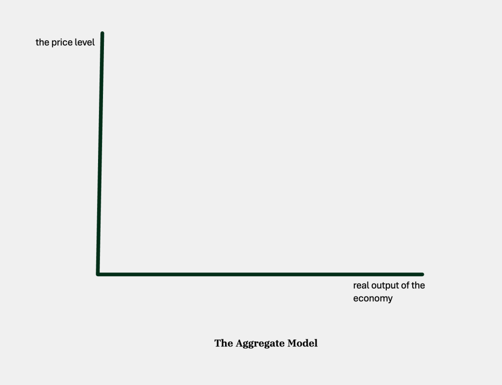
While we have a price variable and a quantity variable on the proper axes, the fact that these are aggregate variables–the price level, not the price of one thing–has important implications. Previously, if the price of our item went up, we talked about substitutes we might switch to. If coffee got more expensive, we might buy more tea. But here, our variable is “the price level”–when coffee is more expensive, so is tea, so is soda, and so is everything else. The meaning of “the price level” is that prices of everything in the economy are moving in the same direction, up or down. So when coffee gets more expensive, you can’t substitute away and buy tea instead.
Notice also the horizontal axis, “real output of the economy.” Instead of one good or service, we are talking about all goods and services that the economy is capable of producing. There will be some point on this axis we will be labelling as “full employment,” the amount of output our economy can optimally produce, given its resources. In the chapter on production and growth, we said the amount we could produce was defined by the production function: Y = t* ƒ (K, H, L, N). We emphasized that Y is real, not nominal. It’s the actual, physical things produced and services being used.
Just looking at the axes of our aggregate model, we see that we are going to be relating something nominal--the price level–with something real, real output. The old-school, classical economists wouldn’t have done this. They would have said that changes in nominal variables–prices–don’t change anything real. By setting up our axes this way, we are saying, maybe nominal can affect real.
The simple versus the aggregate model: the time dimension
Our aggregate model will also introduce a time dimension to the supply-demand landscape. Before, we bought and sold coffee without thinking about time. Our aggregate model will be discussing “the short run” and “the long run.” You might be hoping for a definition in terms of days or years, but that’s not how it works. The short run is now. In the short run, we don’t have full information about everything; we may be confused; we may have wrong information. We didn’t know the printer would need more ink after printing just two pages, or we wouldn’t have bought it. Our expectations may be wrong. We think there’s going to be a lot of price inflation this year, but it turns out, there wasn’t. In the long run, we have full information; we’ve corrected all our misperceptions and wrong expectations. If the long run sounds impossibly perfect–it is. As the famous economist John Maynard Keynes once said, arguing for focussing on the short run, “in the long run, we are all dead.” When we build our aggregate model, we will be using a short run/long run analysis when we build supply curves.
The Aggregate Demand Curve: what happens to each demand sector when the price level is high (the Nightmare World)?
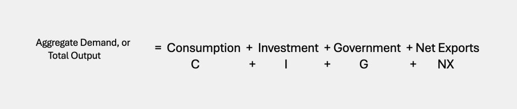
In the chapter where we defined GDP, we divided the parties demanding total GDP into sectors like this:
Now we are going to ask, what happens to aggregate demand from each of these parties when the price level is crazy high, what we called “the Nightmare World”?
First, consumption, C. What happens to your shopping when you walk out of your apartment and everything is very expensive? You get ‘sticker shock’–you try to spend as little as possible. Consumption (C) goes down.
Now, investment, I. When you catch your breath, you go to your broker or bank and decide to sell some bonds, so you’ll have enough liquidity, some cash, to buy lunch! BUT THIS IS HAPPENING TO THE WHOLE ECONOMY! So everyone else is visiting their brokers and trying to sell bonds. When everyone tries to sell bonds, their purchase price has to fall, which means the rate of return on bonds, the interest rate (i) , is pushed up. When the interest rate in the economy is pushed up, Investment (I) goes down. Furthermore, when the interest rate is pushed up, this discourages new home construction, the only ‘consumption’ component of Investment. So Investment (I) falls a second way.
We will hold Government (G) spending constant as a policy variable–later we will be pushing government spending up or down to bring our economy into balance.
Let’s move on to Net Exports (NX). Let’s start with the fact that interest rates (i) in our nightmare economy have been pushed up. When interest rates in our economy are high, bankers in other economies are attracted to buying our bonds. To buy U.S. bonds, they will first sell their Euros, let’s say, for dollars so they can buy some U.S. bonds. All that demand for dollars, pushes up the value of the dollar relative to the Euro. (We call this a ‘strong dollar.’) When the dollar rises in value, U.S. exports start to look expensive to foreigners, since it costs them more of their currencies to purchase our goods. Our exports fall. Meanwhile, with our strong dollar, goods from other countries look cheaper to American consumers–so we buy more imports. When X goes down and M goes up, NX or (X – M) falls.
Bottom line: in the Nightmare World of the high price level, every component of aggregate demand decreased:
| Real Output (Y)= | Consumption (C) | Investment (I) | Government (G) | Net Exports (NX) or (X – M) |
| Price Level High (nightmare world) | decrease (from wealth effect) | decrease
(selling bonds raises i, which lowers I) ( higher i, means new home construction falls) |
held constant as policy variable | decrease
(i goes up, $ stronger, X falls, M rises, so NX falls) |
Aggregate Demand by Components: Y = C + I + G + NX (keep in mind: i = interest rate; I = investment; NX = Exports – Imports)
The Aggregate Demand Curve: what happens to each demand sector when the price level is low (the Fantasy World)?
If we were suddenly in the Fantasy World of a low price level, how would that impact all the components of Aggregate Demand? Let’s take them one by one.
Start with Consumption, C. Imagine you leave your apartment and everything outside is so cheap, you don’t know what to buy first! In the low price level world, your Consumption goes up, what the economists call “the wealth effect.” But maybe you buy everything in sight, and you still have cash in your pocket!
Now we look at what happens to investment, I. With extra cash in your pocket, you head over to your broker and ask her to buy you some bonds! BUT THIS IS HAPPENING TO THE WHOLE ECONOMY! As everyone else also has extra cash, they are there bidding up the purchase price of bonds, causing their rate of return falls. This is equivalent to the interest rate (i) in the economy being pushed down. When the interest rate falls, Investment (I) rises, since it’s now cheaper for businesses to borrow money for expansion. Likewise, consumers decide that a falling interest rate makes it possible to borrow money for new home construction. When home construction, a form of Investment rises, Investment rises a second way.
Again, we hold Government spending, G, constant, as a policy variable.
What happens to Net Exports (NX)? We start with that fall in interest rates. When foreign bankers see that lower interest rate, i, in America, they decide not to buy U.S. bonds. Maybe they buy Euro bonds, because they are paying a higher rate of interest. This will raise demand for Euros relative to dollars, producing a ‘weak dollar.’ American consumers will have to spend more dollars to get a Euro, meaning imports will be more expensive to us, so we will buy less. Imports (M) go down. What happens to our Exports (X)? With the value of the dollar going down and the value of the Euro rising, American goods will look cheaper to shoppers with those strong Euros, so they will buy more American exports. American exports (X) will go up. When X rise and M falls, Net Exports (X-M) will rise.
To summarize: When the price level was low (the Fantasy World), every component of aggregate demand went up:
| Real Output (Y) | Consumption (C) | Investment (I) | Government (G) | Net Exports (NX) or (X – M) |
|
Price Level High (Nightmare world) |
decrease (wealth effect) |
decrease
(selling bonds raises i, which lowers I) higher i, means new home construction falls) |
held constant as policy variable | decrease
(i goes up, $ stronger, X falls, M rises, so NX falls) |
| Price Level Low (Fantasy world) | increase (wealth effect) | increase
(buying bonds lowers i, which raises I) (lower i, means new home construction rises) |
held constant as policy variable | increase
(i goes down, $ weaker, X rises, M falls, so NX rises) |
We see an inverse relationship here between the price level and the quantity of aggregate demand, which we can plot:
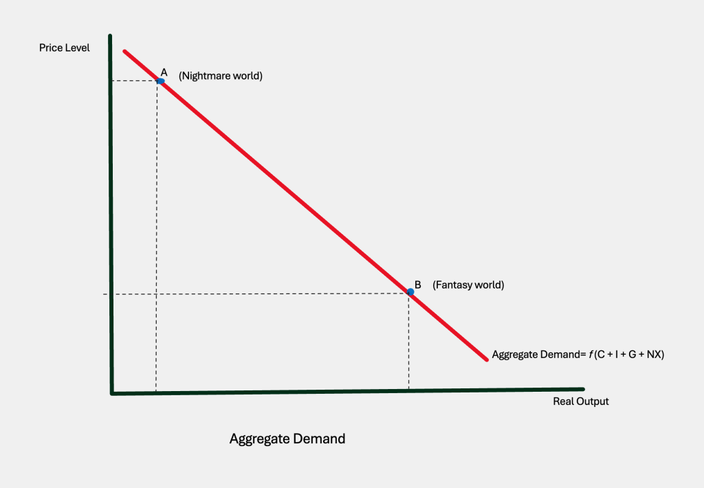
Our Nightmare World (high price level, low aggregate demand) point A and our Fantasy World (low price level, high aggregate demand) point B define a downward-sloping aggregate demand curve. The position of this curve is a function of those components: consumption, investment, government, and net exports. And what determines a curve, is also what will shift it!
What shifts the Aggregate Demand curve?
A curve shifts when any of its determinants shifts, so our aggregate demand curve will be shifted by changes in consumption, investment, government spending or net exports. Let’s see how that looks:
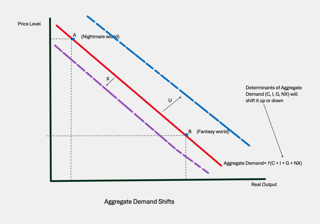
If people are feeling optimistic about the economy, that might increase Consumption (C) which would shift the curve upward or to the right. If there were a depression in Europe, it might decrease their demand for American exports, so our curve would shift downward or to the left. If Investment (I) in America increased, the curve would shift upward, or to the right.
Once again, you use the 3-step method. When some change is proposed, you decide if it is relevant. If yes, ask if that proposed change is the variable on either axis. For example, if the proposed change is an increase in the price level–ok, that’s relevant to aggregate demand, but it is also the variable on the vertical axis. This means you move along a stable curve and you don’t shift anything. But if the change is something impacting consumption, investment, government spending, or the import/export world–you do a shift!
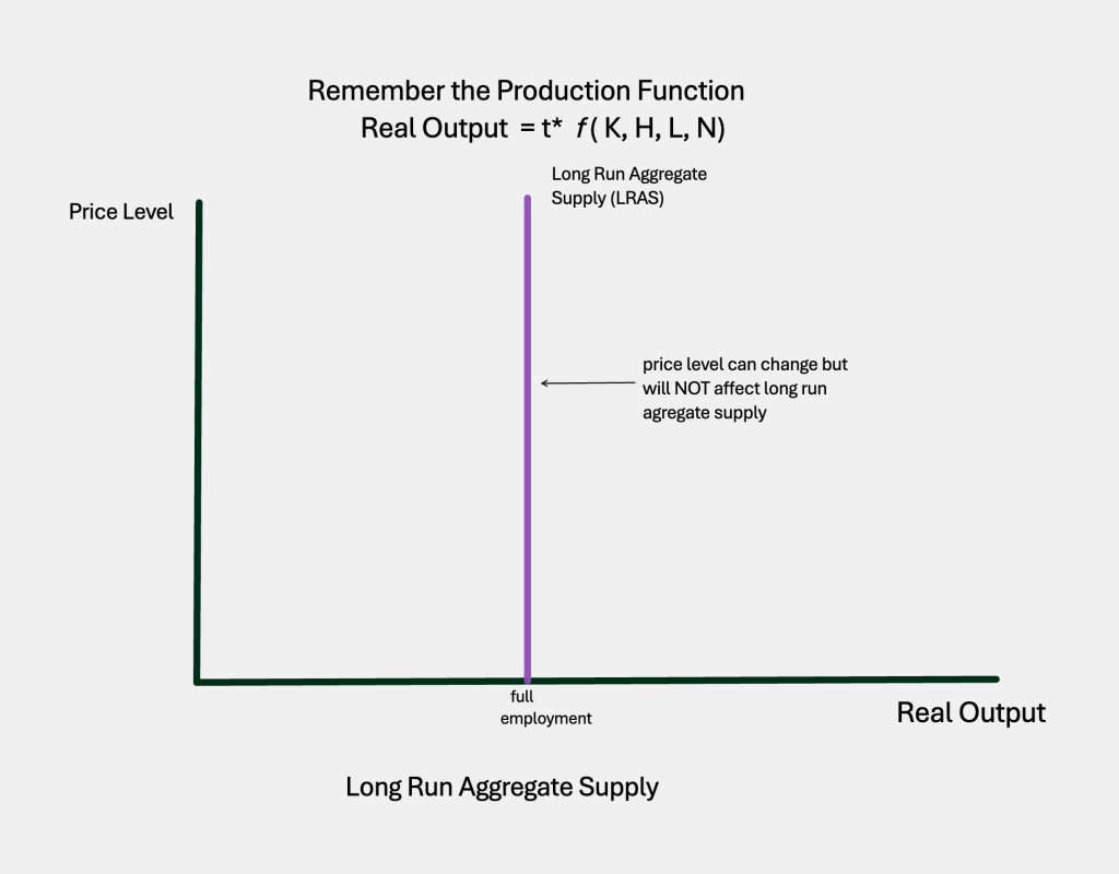
Aggregate supply: the Long Run (LRAS)
With Aggregate Supply, we now have a time dimension–either the short run or the long run. First, let’s talk about the long run, when there’s enough time for all kinds of mistakes and misinformation to be corrected, and enough time for everything to adjust. In this ideal state, the economy can run at its maximum potential, given its resources. This amount that our economy could ideally produce is determined by the production function: Y = t* ƒ(K, H, L, N). (The output of our economy is determined by the amounts of physical capital, human capital, number of workers, and amount of natural resources, all combined at the state-of-the-art technology.) As we learned, the production function is a real relationship, not a nominal one. Changes in the price of eggs or butter don’t change that output of 9 brownies in grandma’s recipe, and changes in the price level do not change the amount of our economy’s output in the long run. This means our Long Run Aggregate Supply (LRAS) curve will be vertical at that level of output:
What will cause the LRAS to shift? Anything that determined where it stands in the first place: t*, K, H, L, and N:
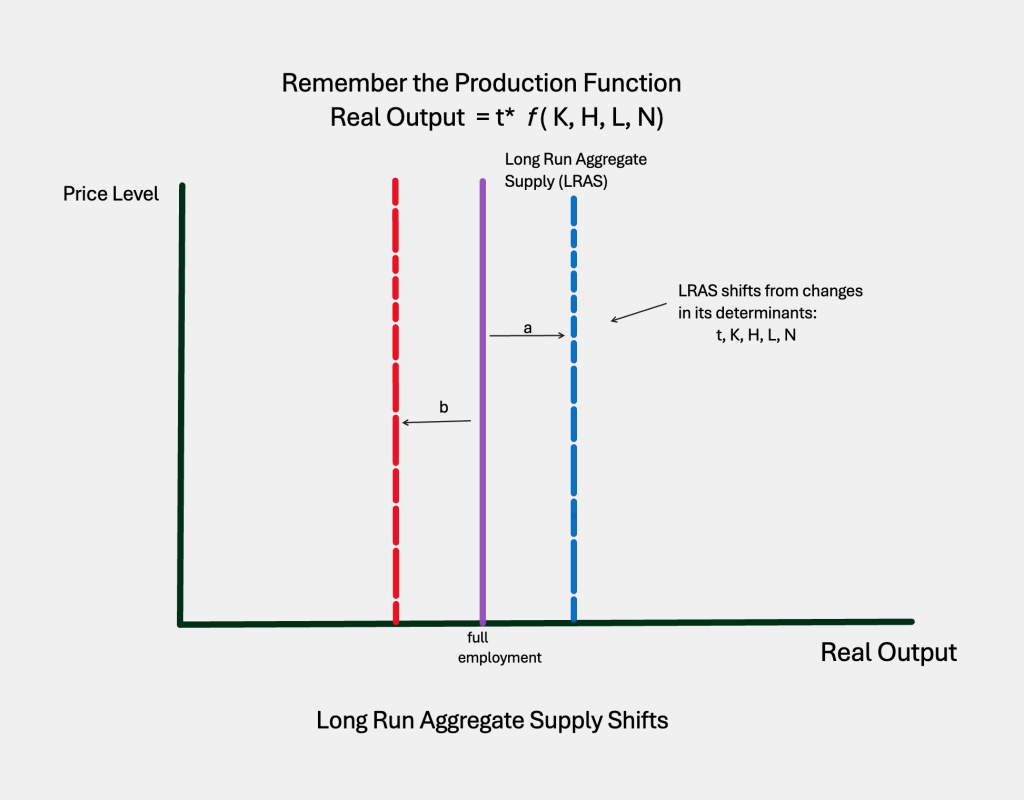
If we improve technology, our LRAS will shift to the right (a). If we shut our borders, decreasing the number of available workers (L) and decreasing the number of ambitious/smart immigrants (H), then the LRAS will shift to the left (b). Even right-wing economists are in favor of immigration!
Aggregate Supply: the short run (SRAS)
In the short run, there is a relationship between the price level and real output. Since it’s easiest to understand this with reference to ‘stickiness’ in input prices, that’s the argument we’ll develop here.
Imagine I own a jeans factory. My three big input costs are labor, cotton, and electricity. To make my business easier, I lock in prices for all three inputs in advance. For example, I sign a 5-year labor contract with my workers, paying $30/hour. I lock in a kilowatt price with the utility company, and a yard goods price for my cotton for the next 5 years as well. Based on my costs, I can charge $60 for my jeans and do fine.
It’s all fine until one morning when I walk to the factory and I realize I’ve entered the Fantasy World of low, low prices. Everything’s cheap! I’m as happy as anyone else, until I think about my jeans priced at $60. I can’t sell jeans for $60 when a whole dinner costs $1-2. I’m going to have to mark down my jeans to $30. After I cut my prices in the showroom, I go back to the workroom to tell my workers their wage has to go down as well. The workers say yes…in five years, when our contract expires! I go to my office so I can call the utility company and the cotton dealer and get a cost cut–but I get the same answer from them! In five years, when our contracts end, I can negotiate for cheaper input prices. My situation is not good–my jeans are selling for half of their previous price, but my input costs are sticky, they have not gone down. In the short run–for the next five years–my profit margin is so small-to-negative that I want to produce as little as possible.
Let’s try a different scenario. Suppose, walking to work, I discovered I’d stepped into the Nightmare World of high, high prices. People are paying $20 for a subway ride. Aren’t my jeans worth more than 3 subway rides? When I get to my showroom, I mark up all my jeans from $60 to $120. But when I go back to the workroom, everyone is grumpy. They tell me $30/hr is no longer a living wage, when it costs $20 for a single subway ride. They want raises! I tell them they’ll get a raise–in 5 years! I retreat to my office to escape their complaints, only to hear the phone ringing like crazy. The utility company and the cotton dealer both want to charge me more, which…I’ll allow in 5 years! Looking at my spreadsheet, I realize that with a higher market price on the jeans, but no increase in input costs, my profit margin on each pair produced is huge. I want to produce as much as possible.
Bottom line–in the short run, when the price level was low, I wanted to produce very little (point A below). When the price level was high, I wanted to produce a lot (point B below). This would be true, in this example, for five years. After that, everything could adjust freely, without those contracts preventing changes in input pricing. These legal contracts are a type of “stickiness,” preventing all prices from adjusting instantly, the way they would in the long run:
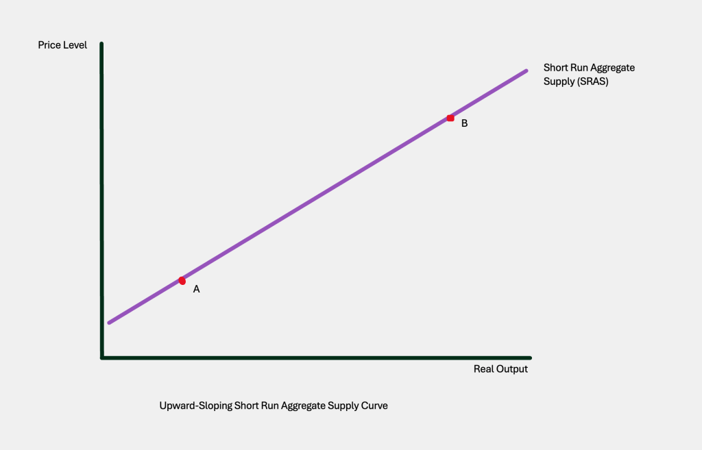
There are other explanations for an upward-sloping SRAS–inflation expectations, misperceptions–but one’s enough for us. Now that we have all three of our aggregate curves, it’s time to put them together.
Some Useful Materials
Watch the first of 2 videos on aggregate demand.
Watch the second video on aggregate demand, which discusses shifts in the curve.
Watch a video on the LRAS (long run aggregate supply) curve.
Watch a video on the SRAS (short run aggregate supply) curve.
Watch a very British video on the aggregate model, giving a slightly different take!
Media Attributions
- patrick-pellegrini–z9qR62Xulw-unsplash © Patrick Pellegrini
- simple aggregate axes © Bettina Berch is licensed under a CC BY-NC (Attribution NonCommercial) license
- components of agg demand © Bettina Berch is licensed under a CC BY-NC (Attribution NonCommercial) license
- Agg Demand © Bettina Berch is licensed under a CC BY-NC (Attribution NonCommercial) license
- Aggregate D shifts © Bettina Berch is licensed under a CC BY-NC (Attribution NonCommercial) license
- LRAS © Bettina Berch is licensed under a CC BY-NC (Attribution NonCommercial) license
- LRAS shifts © Bettina Berch is licensed under a CC BY-NC (Attribution NonCommercial) license
- SRAS © Bettina Berch is licensed under a CC BY-NC (Attribution NonCommercial) license
