Module 6: Probability and Probability Distributions
Normal Random Variables (2 of 6)
Normal Random Variables (2 of 6)
Learning OUTCOMES
- Use a normal probability distribution to estimate probabilities and identify unusual events.
Example
Beyond One Standard Deviation from the Mean
Earlier we stated that for all normal curves, the area within 1 standard deviation of the mean will equal 0.68. From this fact, we can see that the area outside of this region equals 1 − 0.68 = 0.32. And since normal curves are symmetric, this outside area of 0.32 is evenly divided between the two outer tails. So the area of each tail = 0.16.
[latex]\text{area of each tail} = \frac{1}{2}(1 - \text{central area}) = \frac{1}{2}(1 - .68) = \frac{1}{2}(.32) = .16[/latex]
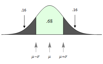
The outer tail areas allow us to answer related probability questions:
- Question: What is the probability that a normal random variable is more than 1 standard deviation from its mean?
- Answer: 0.32
- Question: What is the probability that a normal random variable is more than 1 standard deviation larger than its mean?
- Answer: 0.16
Before leaving this example, we highlight one more geometric fact about normal curves. Look at the arrows pointing at the normal curve in the following figure.
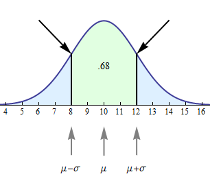
At these points, the curve changes the direction of its bend and goes from bending upward to bending downward, or vice versa. A point like this on a curve is called an inflection point. Every normal curve has inflection points at exactly 1 standard deviation on each side of the mean.
With the following simulation, you can look at a variety of normal curves. Use the slider to change the standard deviation. As you change the standard deviation, you will of course get different normal curves. Observe that the two properties we discussed in the examples remain true for any standard deviation you select:
- The probability that a value is within 1 standard deviation of the mean is 68%.
- The x-values of the inflection points correspond to 1 standard deviation above and below the mean.
Click here to open this simulation in its own window.
Try It
Now we extend this idea to look at the probability of a value falling within 2 standard deviations of the mean or 3 standard deviations of the mean.
If X is a normal random variable with mean μ and standard deviation σ, then
- The probability that X is within 1 standard deviation of the mean equals approximately 0.68.
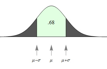
- The probability that X is within 2 standard deviations of the mean equals approximately 0.95.
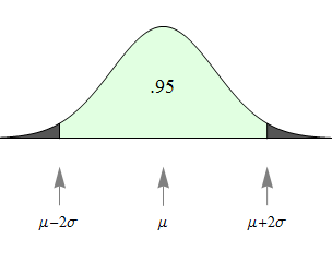
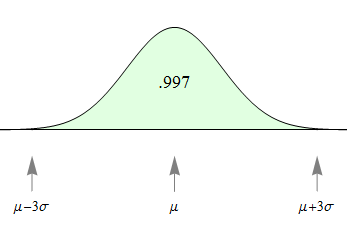
- The probability that X is within 3 standard deviations of the mean equals approximately 0.997.
To summarize using probability notation:
- [latex]P(\mu - \sigma < X < \mu + \sigma) = 0.68[/latex]
- [latex]P(\mu - 2\sigma < X < \mu + 2\sigma) = 0.95[/latex]
- [latex]P(\mu - 3\sigma < X < \mu + 3\sigma) = 0.997[/latex]
These three facts together are called the empirical rule for normal curves.
Comment
Let’s take a moment to look a bit deeper at what the empirical rule tells us.
- The first statement of the empirical rule really defines a range of likely values of X. It gives us an interval – within 1 standard deviation of the mean – that contains the central 68% of the values. This statement is very similar to statements about the interquartile range (IQR) that we saw back in the module Summarizing Data Graphically and Numerically. The IQR is the width of the interval that captures the central 50% of the data points of a quantitative distribution.
- The second and third statements in the empirical rule help us identify values that are unlikely to occur. Compare this to the discussion in Summarizing Data Graphically and Numerically where we defined an outlier to be a value that is either more than 1.5 IQRs above quartile 3 or more than 1.5 IQRs below quartile 1. Here we can make the following characterizations of extreme values in normal distributions.
- 95% of values fall within 2 standard deviations of the mean. It is therefore unlikely for a value to fall more than 2 standard deviations away from the mean. Values more than 2 standard deviations away from the mean in a normal distribution are often called outliers.
- 99.7% of values fall within 3 standard deviations of the mean. It is therefore extremely unlikely for a value to fall more than 3 standard deviations away from the mean. Values more than 3 standard deviations away from the mean are often called extreme outliers.
Try It
1. The second statement of the Empirical Rule (in both words and symbols) is:
The probability that X is within 2 standard deviations of the mean equals approximately 0.95.
[latex]P(\mu - 2\sigma < X < \mu + 2\sigma) = 0.95[/latex] Use this to find the area of each tail indicated by the question marks in the image below.
2. The third statement of the Empirical Rule (in both words and symbols) is:
The probability that X is within 3 standard deviations of the mean equals approximately 0.997.
[latex]P(\mu - 3\sigma < X < \mu + 3\sigma) = 0.997[/latex] Use this to find the area of each tail indicated by the question marks in the image below.
- Concepts in Statistics. Provided by: Open Learning Initiative. Located at: http://oli.cmu.edu. License: CC BY: Attribution
