Module 9: Inference for Two Proportions
Distribution of Differences in Sample Proportions (1 of 5)
Distribution of Differences in Sample Proportions (1 of 5)
Learning outcomes
- Describe the sampling distribution of the difference between two proportions.
- Draw conclusions about a difference in population proportions from a simulation.
Our goal in this module is to use proportions to compare categorical data from two populations or two treatments.
It’s not about the values – it’s about how they are related!
In Inference for One Proportion, we learned to estimate and test hypotheses regarding the value of a single population proportion. Here, in Inference for Two Proportions, the value of the population proportions is not the focus of inference. Instead, we want to develop tools comparing two unknown population proportions.
The first step is to examine how random samples from the populations compare. In this investigation, we assume we know the population proportions in order to develop a model for the sampling distribution. This is the same thinking we did in Linking Probability to Statistical Inference. In that module, we assumed we knew a population proportion. Then we selected random samples from that population. We examined how sample proportions behaved in long-run random sampling. This is the same approach we take here.
Example
Teen Depression
Most of us get depressed from time to time. Depression is a normal part of life. Many people get over those feelings rather quickly. But some people carry the burden for weeks, months, or even years. For these people, feelings of depression can have a major impact on their lives. Depression can cause someone to perform poorly in school or work and can destroy relationships between relatives and friends.
Research suggests that teenagers in the United States are particularly vulnerable to depression. And, among teenagers, there appear to be differences between females and males. The Christchurch Health and Development Study (Fergusson, D. M., and L. J. Horwood, “The Christchurch Health and Development Study: Review of Findings on Child and Adolescent Mental Health,” Australian and New Zealand Journal of Psychiatry 35[3]:287–296), which began in 1977, suggests that the proportion of depressed females between ages 13 and 18 years is as high as 26%, compared to only 10% for males in the same age group.
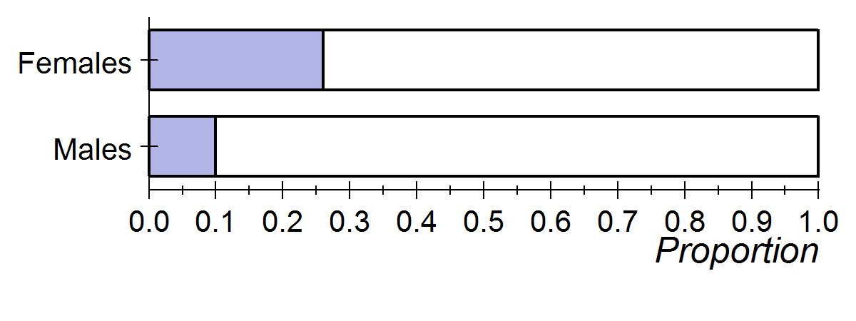
Let’s assume that 26% of all female teens and 10% of all male teens in the United States are clinically depressed. In other words, assume that these values are both population proportions.
- pf = 0.26 for the population of all female teenagers in the United States
- pm = 0.1 for the population of all male teenagers in the United States
Graphically, we can compare these proportion using side-by-side ribbon charts:

To compare these proportions, we could describe how many times larger one proportion is than the other. Here the female proportion is 2.6 times the size of the male proportion (0.26/0.10 = 2.6). An easier way to compare the proportions is to simply subtract them. This is the approach statisticians use. The difference between the female and male proportions is 0.16. This is a 16-percentage point difference. We write this with symbols as follows:
[latex]p_{f} -p_{m}[/latex] = 0.26 − 0.10 = 0.16
Another study, the National Survey of Adolescents (Kilpatrick, D., K. Ruggiero, R. Acierno, B. Saunders, H. Resnick, and C. Best, “Violence and Risk of PTSD, Major Depression, Substance Abuse/Dependence, and Comorbidity: Results from the National Survey of Adolescents,” Journal of Consulting and Clinical Psychology 71[4]:692–700) found a 6% higher rate of depression in female teens than in male teens. Suppose that this result comes from a random sample of 64 female teens and 100 male teens. Let’s assume that 9 of the females are clinically depressed compared to 8 of the males. The proportion of females who are depressed, then, is 9/64 = 0.14. The proportion of males who are depressed is 8/100 = 0.08. The difference between the female and male sample proportions is 0.06, as reported by Kilpatrick and colleagues. We write this with symbols as follows:
[latex]\hat{p} _{f} -\hat{p}_{m}[/latex] = 0.14 − 0.08 = 0.06
Of course, we expect variability in the difference between depression rates for female and male teens in different studies. But does the National Survey of Adolescents suggest that our assumption about a 0.16 difference in the populations is wrong? Or could the survey results have come from populations with a 0.16 difference in depression rates? Does sample size impact our conclusion?
Try It
We will use a simulation to investigate these questions. The simulation will randomly select a sample of 64 female teens from a population in which 26% are depressed and a sample of 100 male teens from a population in which 10% are depressed. (In the real National Survey of Adolescents, the samples were very large. Later we investigate whether larger samples will change our conclusion.)
A simulation is needed for this activity. Click here to open this simulation in its own window.
Click here to open this simulation in its own window.
Try It
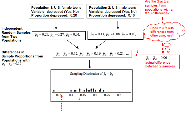
This diagram illustrates our process here. Notice that we are sampling from populations with assumed parameter values, but we are investigating the difference in population proportions. From the simulation, we can judge only the likelihood that the actual difference of 0.06 comes from populations that differ by 0.16. We cannot make judgments about whether the female and male depression rates are 0.26 and 0.10 respectively. We can make a judgment only about whether the depression rate for female teens is 0.16 higher than the rate for male teens. This is what we meant by “It’s not about the values – it’s about how they are related!”

- Concepts in Statistics. Provided by: Open Learning Initiative. Located at: http://oli.cmu.edu. License: CC BY: Attribution
