Module 9: Inference for Two Proportions
Estimate the Difference between Population Proportions (1 of 3)
Estimate the Difference between Population Proportions (1 of 3)
Learning outcomes
- Recognize when to use a hypothesis test or a confidence interval to compare two population proportions or to investigate a treatment effect for a categorical variable.
- Construct a confidence interval to estimate the difference between two population proportions (or the size of a treatment effect) when conditions are met. Interpret the confidence interval in context.
In “Distributions of Differences in Sample Proportions,” we used simulation to observe the behavior of the differences in sample proportions when we randomly select many, many samples. From the simulation, we developed a normal probability model to describe the sampling distribution of sample differences. With this model, we are now ready to do inference about a difference in population proportions (or about a treatment effect.)
When our goal is to estimate a difference between two population proportions (or the size of a treatment effect), we select two independent random samples and use the difference in sample proportions as an estimate. Of course, random samples vary, so we want to include a statement about the amount of error that may be present. Because the differences in sample proportions vary in a predictable way, we can also make a probability statement about how confident we are in the process that we used to estimate the difference between the population proportions. You may recognize that what we are describing is a confidence interval.
In Inference for One Proportion, we calculated confidence intervals to estimate a single population proportion. In this section, “Estimate the Difference between Population Proportions,” we learn to calculate a confidence interval to estimate the difference between two population proportions. If the data comes from an experiment, we estimate the size of the treatment effect.
Try It
Confidence Interval for a Difference in Two Population Proportions: the Basics
Every confidence interval has this form:
statistic ± marginoferror
To estimate a difference in population proportions (or a treatment effect), the statistic is a difference in sample proportions, so the confidence interval is
(differenceinsampleproportions) ± marginoferror
When we select two random samples and calculate the difference in the sample proportions, we do not know the exact amount of error for this particular pair of samples. We therefore use the standard error as a typical amount of error and calculate the margin of error from the standard error, as we did in Inference for One Proportion.
If a normal model is a good fit for the sampling distribution, we can use it to make probability statements that describe our confidence in the interval. More specifically, we use the normal model to describe our confidence that the difference in population proportions lies within a given margin of error of the difference in sample proportions. For example, we can state that we are 95% confident that the difference in population proportions is contained in the following interval:
(differenceinsampleproportions) ± 2 (standarderror)
Try It
Nuclear Power
The following problem is based on a report, “Opposition to Nuclear Power Rises amid Japanese Crisis,” by the Pew Research Center (March 21, 2011).
After the nuclear reactor accidents in Japan during the spring of 2011, there was a shift in public support for expanded use of nuclear power in the United States. A few months before the accident, 47% of a random sample of 1,004 U.S. adults supported expanded use of nuclear power. After the nuclear accident in Japan, 39% of a different random sample of 1,004 U.S. adults favored expanded use.
What Does 95% Confident Really Mean?
95% confident comes from a normal model of the sampling distribution.
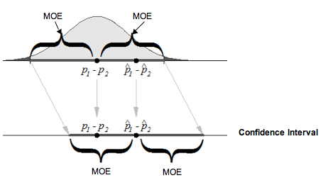
To review this idea in the context of differences in sample proportions, let’s start with a picture to help us visualize a confidence interval and its relationship to the sampling distribution. The following normal model represents the sampling distribution.

In the diagram, notice the sample difference. In the sampling distribution, we can see that the error in this sample difference is less than the margin of error. We know this because the distance between the sample difference and the population difference is shorter than the length of the margin of error (abbreviated MOE in the figure). When we create a confidence interval with this sample difference, we mark a distance equal to a margin of error on either side of the sample difference. Notice that this interval contains the population difference, which makes sense because the distance between the population difference and the sample difference has not changed.
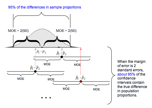
So where does the “95%” come from? If the normal model is a good fit for the sampling distribution, then the empirical rule applies. The empirical rule says that 95% of the values in a normal distribution fall within 2 standard deviations of the mean. So 95% of the sample differences are within 2 standard errors of the mean difference. Remember that the mean difference is the difference in population proportions. Now consider the confidence interval centered at a sample difference. From the empirical rule, it follows that 95% of the confidence intervals, with a margin of error equal to 2 standard errors, will contain the population difference.
Following is another illustration of 95% confidence, a concept that is often misinterpreted. This diagram helps us remember the correct interpretation. If we construct confidence intervals with a margin of error equal to 2 standard errors, then 95% confidence means that in the long run, 95% of these confidence intervals will contain the population difference, and 5% of the time, the interval we calculate will not contain it. We show one of these less common intervals with a red dot at the sample difference.

Of course, in reality, we don’t know the difference in population proportions. (This is the why we want to estimate it with a confidence interval!) So, in reality, we will not be able to determine if a specific confidence interval does or does not contain the true difference in population proportions. This is why we state a level of confidence. For a specific interval, we say we are 95% confident that the interval contains the true difference in population proportions.
Example
Correct and Incorrect Interpretations of 95% Confidence
Recall our earlier example about the change in public opinion after the nuclear accident in Japan. We concluded, “We are 95% confident that there was a 4% to 12% drop in support for the expanded use of nuclear power in the United States after the nuclear accident in Japan.”
Here are some accurate ways to describe the phrase “95% confident” for this confidence interval:
- There is a 95% chance that poll results from two random samples will give a confidence interval that contains the true change in public support for the expanded use of nuclear power in the United States after the nuclear accident in Japan
- 95% of the time, this method produces an interval that covers the true difference in the proportions of the U.S. adult population supporting expanded use of nuclear power in the United States before and after the nuclear accident in Japan.
Here are some incorrect interpretations:
- There is a 95% chance that the true difference in public opinion (before and after the nuclear accident in Japan) is between 4% and 12%.
- There is a 95% chance that there was a 4% to 12% drop in support for the expanded use of nuclear power in the United States after the nuclear accident in Japan.
What do you notice? In the correct interpretations, the 95% is a probability statement about the random event of sampling. So statements like “95% chance that two random samples give a confidence interval” and “95% of the time, this method produces an interval” describe the chance that confidence intervals, in the long run, contain the difference in population proportions.
In the wrong interpretations, the phrase “95% chance” is a probability statement about the specific interval 4% to 12%. Since we already found the confidence interval, there is no random event in this description, so we cannot make a probability statement about a single specific interval. For this reason, we use the phrase “95% confident” when we are describing a single interval from a specific study.
Try It
- Concepts in Statistics. Provided by: Open Learning Initiative. Located at: http://oli.cmu.edu. License: CC BY: Attribution
