Normal Random Variables (3 of 6)

Normal Random Variables (3 of 6)

Learning OUTCOMES

• Use a normal probability distribution to estimate probabilities and identify unusual events.

Example

The Empirical Rule in a Context

Suppose that foot length of a randomly chosen adult male is a normal random variable with mean μ = 11 and standard deviation σ = 1.5. Then the empirical rule lets us sketch the probability distribution of X as follows:

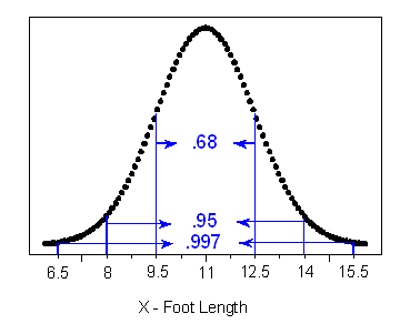
• (a) What is the probability that a randomly chosen adult male will have a foot length between 8 and 14 inches?
• Answer: 0.95, or 95%
• (b) An adult male is almost guaranteed (0.997 probability) to have a foot length between what two values?
• Answer: 6.5 and 15.5 inches
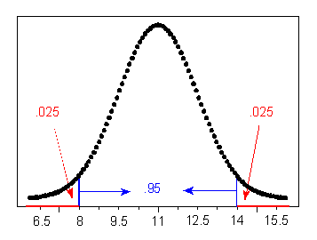
• (c) The probability is only 2.5% that an adult male will have a foot length greater than how many inches?
• Answer: 14 inches

Ninety-five percent of the area is within 2 standard deviations of the mean, so 2.5% of the area is in the tail above 2 standard deviations. The x-value 2 standard deviations above the mean is 14 inches.

Now you should try a few: questions (d), (e), and (f) are presented in the Try It activity. Use the figure preceding question (a) to help you.

Try It

Comment

Notice that there are two types of problems we may want to solve: those like (a) and, from the Try It activity, (d) and (e), in which a particular interval of values of a normal random variable is given and we are asked to find a probability; and those like (b), (c), and, from the Try It, (f), in which a probability is given and we are asked to identify values of the normal random variable.

CC licensed content, Shared previously

• Concepts in Statistics. Provided by: Open Learning Initiative. Located at: http://oli.cmu.edu. License: CC BY: Attribution

Feedback for interactive question
(d) How likely or unlikely is a male’s foot length to be smaller than 9.5 inches? Not too unlikely, since the probability of being smaller than 9.5 is 0.16, which is not a particularly low probability.

Feedback: Indeed, the probability that foot length is between 9.5 and 12.5 is 0.68, and therefore the remaining two tails together have probability 1 − 0.68 = 0.32. We conclude, then, that: P(X 15.5) = 0.003/2 = 0.0015.

(e) How likely or unlikely is a foot length longer than 15.5 inches? Extremely unlikely, since the probability of being longer than 15.5 is only 0.0015.

Feedback: Indeed, the probability that foot length is between 6.5 and 15.5 is 0.997, and therefore the remaining two tails together have probability 1 − 0.997 = 0.003. We conclude, then, that P(X > 15.5) = 0.003/2 = 0.0015.

(f) There is probability of 0.5 that a male’s foot is shorter than 11.

Feedback: The value that divides the area under the curve into two halves is 11, so that P(X 11) = 0.5.