Estimating a Population Mean (3 of 3)

Structure of a Confidence Interval

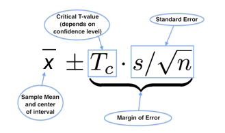
Let’s take a closer look at the parts of the confidence interval. Remember that this is a confidence interval for a population mean. We use this formula when the population standard deviation is unknown.

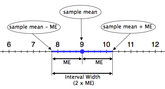
Let’s remind ourselves how the confidence interval formula relates to the graph of the confidence interval on a number line.

The confidence interval shown below is a 95% confidence interval for a sample of size n = 25 (so df = 24), with sample mean [latex]\bar{x}[/latex]= 9 and sample standard deviation of s = 3. The critical T-value for a 95% confidence interval with a df = 24 is 2.064.

Standard error is [latex]3/\sqrt{25}=0.6[/latex]

Martin of error (ME) is [latex]2.064(3)/\sqrt{25}≈ 1.24[/latex]

The confidence interval is 9 ± 1.24. We are 95% confident that µ lies between 7.76 and 10.24.

Note:

• The sample mean (9 in this example) is at the center of the interval.
• The margin of error (labeled ME and equal to 1.24 in this example) is the distance that the interval extends to the left and right of the sample mean.
• The interval width is the length of the entire interval on the number line. The interval width is always twice the margin of error.

Let’s quickly review how the precision of a confidence interval relates to the margin of error:

• An interval gives a more precise estimate when the interval is narrower. In other words, the margin of error is smaller.
• An interval gives a less precise estimate when the interval is wider. In other words, the margin of error is larger.

We know that a higher confidence level gives a larger margin of error, so confidence level is also related to precision.

• Increasing the confidence in our estimate makes the confidence interval wider and therefore less precise.
• Decreasing the confidence in our estimate makes the confidence interval narrower, and therefore more precise.

Confidence interval estimates are useful when they have the right balance of confidence and precision. Typical confidence levels used in practice are 90%, 95%, and 99%. When we need to be really sure about our estimates, such as in life-and-death situations, we choose a 99% confidence level. So if nothing else changes, we settle for less precise estimates when we need a high level of confidence.

In our discussion about the structure of confidence intervals, we said choosing a higher level of confidence means that we sacrifice some precision. This is true only if nothing else changes. But there is one way to keep a high level of confidence without sacrificing precision: Increase the sample size. We investigate the impact of sample size on the confidence interval next.

Example

Cable Strength Revisited

Recall the engineers who are trying to determine the breaking weight of a cable. In that example, we had a random sample of 45 cables with a mean breaking weight of 768.2 lb and a standard deviation of 15.1 lb. From that sample we computed a 95% confidence interval for the mean breaking weight of all such cables. Here are the important numbers we found from that calculation on the previous page:

standard error: [latex]\textit{s}/\sqrt{n} = 15.1/\sqrt{45}[/latex] ≈ 2.25

critical T-value: T_c = 2.015 (we found this using the simulation)

margin of error: T_c · s/[latex]\sqrt{n}[/latex] =2.015(2.25)=4.53

confidence internal: 768.2±4.53 or (763.67, 772.73)

Now let’s increase the sample size and investigate the impact on the confidence interval. We calculate the confidence interval for a larger sample of 101 cables (n = 101).

Sample size affects our calculations in two ways:

• The sample size (n) appears in our formula for standard error.
• The critical T-value depends on degrees of freedom, and df = n – 1.

Finding the standard error:

We approximate the standard error of all sample means as follows:

[latex]\textit{s}/\sqrt{n}[/latex] = 15.1/[latex]\sqrt{101}[/latex] ≈ 1.50

Note: The standard error is smaller when the sample size is larger. We were expecting this because we know there is less variability in sample means when the samples are larger.

Finding the critical T-value:

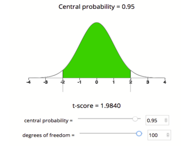
To find the critical T-value, we use the simulation. We set the df to 100 and the central probability to 0.95. We see that the critical T-value is 1.984.

Note: Increasing the sample size decreased the critical T-value (the T-value went from 2.015 to 1.984 when we increased the sample size). You might also notice that both of the critical T-values for 95% confidence are larger than the critical Z-value for 95% confidence, which is approximately 1.96. This makes sense because the T-models are wider than the the standard normal curve.

Finding the margin of error.

Here is the margin of error calculation:

T_c · s/[latex]\sqrt{n}[/latex] = 1.984(1.50) = 2.98

Finding the confidence interval.

Here is the confidence interval calculation:

[latex]\bar{x}[/latex] ± margin of error

[latex]\bar{x}[/latex] ± T_c · [latex]\frac{s}{\sqrt{n}}[/latex]

768.2±2.98

(765.22, 771.18)

Side-by-side comparison:

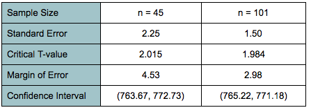
Let’s take a look at these two intervals to study the effects of changing the sample size.

Increasing the sample size had the following effects on the confidence interval estimate:

• Decreased standard error
• Decreased critical T-value
• Decreased margin of error and hence decreased the interval width
• Improved interval precision

Comment

In the real world, increasing the sample size is not always possible. Sometimes collecting a sample is very expensive. If the study has budgetary constraints, which is usually the case, selecting a larger sample may be too expensive.

Let’s Summarize

• A confidence interval approximates a population mean by giving us a range of values that likely contains the population mean, μ. The general form of the confidence interval is [latex]\bar{x}[/latex] ± margin of error.
• To say that we are “95% confident that the population mean falls within our confidence interval” really means that “about 95% of all confidence intervals computed in this way will capture the true population mean.”
• We can use a sample mean to build a confidence interval as an estimate for μ. There are two possible cases:
  • Suppose the population standard deviation, σ, is known. We check the conditions for use of the normal model. Conditions: The variable must be normally distributed in the population, or the sample size is large enough (n > 30). In this case, the confidence interval has the form [latex]\bar{x} \pm Z{c}\cdot \sigma/\sqrt{n}[/latex].
  • Suppose the population standard deviation, σ, is not known. Then we use the sample standard deviation, s, as an approximation for σ. We check the conditions for use of the T-model. Conditions are the same: The variable must be normally distributed in the population, or the sample size is large enough (n > 30). In this case, the confidence interval has the form [latex]\bar{x} \pm T{c}\cdot s/\sqrt{n}[/latex]. When using the T-model to find the critical value, we need to select an appropriate number of degrees of freedom (df). The number of degrees of freedom is 1 less than the sample size (df = n – 1).
• As we have seen with other confidence intervals, the width of a confidence interval is twice the margin of error. The smaller the margin of error, the more narrow the confidence interval and the more precise the estimate of µ.