Assessing the Fit of a Line (3 of 4)

Introduction

Here we continue our discussion of the question, How good is the best-fit line?

Let’s summarize what we have done so far to address this question. We began by looking at how the predictions from the least-squares regression line compare to observed data. We defined a residual to be the amount of error in a prediction. Next, we created residual plots. A residual plot with no pattern reassures us that our linear model is a good summary of the data.

But how do we know if the explanatory variable we chose is really the best predictor of the response variable?

The regression line does not take into account other variables that might also be good predictors. So let’s investigate the question, What proportion of the variation in the response variable does our regression line explain?

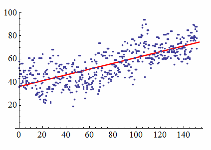
We begin our investigation with a scatterplot of the daily high temperature (°F) in New York City from January 1 to June 1. We have 4 years of data (2002, 2003, 2005, and 2006). The least-squares regression line has the equation y = 36.29 + 0.25x, where x is the number of days after January 1. Therefore, January 1 corresponds to x = 0, and June 1 corresponds to x = 151.

Two things stand out as we look at this picture. First, we see a clear, positive linear relationship tracked by the regression line. As the days progress, there is an associated increase in temperature. Second, we see a substantial scattering of points around the regression line. We are looking at 4 years of data, and we see a lot of variation in temperature, so the day of the year only partially explains the increase in temperature. Other variables also influence the temperature, but the line accounts only for the relationship between the day of the year and temperature.

Now we ask the question, Given the natural variation in temperature, what proportion of that variation does our linear model explain?

The answer, which is surprisingly easy to calculate, is just the square of the correlation coefficient.

The value of r² is the proportion of the variation in the response variable that is explained by the least-squares regression line.

In the present case, we have r = 0.73; therefore, [latex]\frac{\text{explained variation}}{\text{total variation}} = 0.73^2 = 0.53[/latex]. And so we say that our linear regression model explains 53% of the total variation in the response variable. Consequently, 47% of the total variation remains unexplained.

Example

Highway Sign Visibility

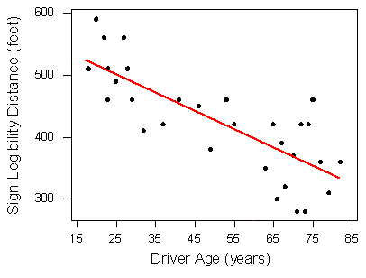
Recall that the least-squares regression line is Distance = 576 − 3 * Age. The correlation coefficient for the highway sign data set is −0.793, so r² = (−0.793)² = 0.63.

Our linear model uses age to predict maximum distance at which a driver can read a highway sign. Other variables may also influence reading distance. We can say the linear relationship between age and maximum reading distance accounts for 63% of the variation in maximum reading distance.