Module 3: Examining Relationships: Quantitative Data
Assessing the Fit of a Line (4 of 4)
Assessing the Fit of a Line (4 of 4)
Learning OUTCOMES
- Use residuals, standard error, and r2 to assess the fit of a linear model.
Introduction
Our final investigation into assessing the fit of the regression line focuses on typical error in the predictions.
Previously, we calculated the error in a single prediction by calculating
Residual = Observed value − Predicted value
But we use the regression line to make predictions even when we do not have an observed value, so we need a method for using all of the residuals to compute a typical amount of error.
We ask the question, How do we measure the typical amount of error for predictions from the regression line?
The most common measure of the size of the typical error is the standard error of the regression, which is represented by se. It is calculated using the following formula:
[latex]s_e = \sqrt{\frac{\text{SSE}}{n - 2}}[/latex]
where SSE stands for the sum of the squared errors.
Finding the standard error of the regression is similar to finding the standard deviation of a distribution of data points from a single quantitative variable. In Summarizing Data Graphically and Numerically, we learned that the standard deviation is roughly a measure of average distance about the mean. Here the standard error is roughly a measure of the average distance of the points about the regression line.
Let’s return to our example where age is used to predict the maximum distance for reading highway signs.
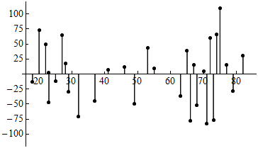
The residual plot for the highway sign data set is shown below. We can visualize the SSE in the formula as simply the sum of the squares of all of the vertical (residual) line segments. After dividing by n − 2, we have the average squared residual. Taking the square root then gives us a measure of the average size of the residuals.

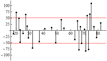
In the case of the highway sign data, the value of se is 51.35. In the figure below, we added horizontal lines at y = 51.35 and y = −51.35, so the red line represents the typical size of the error.

Comment: When we mark the se on this residual plot, errors that fall outside of this range are larger than average. We see again that most of the errors that exceed ±51.35 are on the right. This illustrates that predictions of maximum reading distance for older drivers have larger error.
Note: Most statistics software computes r and r2 and se. Therefore, our focus is not on calculating but on understanding and interpreting.
Now let’s apply the standard error of the regression as a measurement of typical error.
Example
Highway Sign Visibility
Let’s take another look at the prediction we made earlier using the regression line equation:
Distance = 576 + (−3 * Age)
In a previous example, we predicted the maximum distance that a 60-year-old driver can read a highway sign. We plugged Age = 60 into the equation and found that
Predicted distance = 576 + (−3 * 60) = 396
The question we now ask is, How good is this prediction?
Unfortunately, there is no 60-year-old driver in the original data set of 30 drivers, so we cannot calculate the residual. Instead, we use the se as a measurement of typical error.
Technology gives se = 51.35.
So how good is the prediction for the 60-year-old driver? Based on the se for this data, we estimate that our prediction of 396 feet is off by ±51 feet.
| Intro grade(%) | Upper grade(%) | Predictions | Error (Residual) | Error Squared | |
| Student 1 | 65 | 58 | 59.1 | −1.1 | 1.21 |
| Student 2 | 71 | 63 | 65.4 | −2.4 | 5.76 |
| Student 3 | 72 | 67 | 66.4 | 0.6 | 0.36 |
| Student 4 | 72 | 77 | 66.4 | 10.6 | 112.36 |
| Student 5 | 75 | 63 | 69.6 | −6.6 | 43.56 |
| Student 6 | 83 | 72 | 77.9 | −5.9 | 34.81 |
| Student 7 | 85 | 84 | 80 | 4 | 16 |
| Student 8 | 88 | 83 | 83.2 | −0.2 | 0.04 |
| Student 9 | 94 | 89 | 89.5 | −0.5 | 0.25 |
| Student 10 | 96 | 93 | 91.5 | 1.5 | 2.25 |
Try It
Try It
Let’s Summarize
- When we use a regression line to make predictions, there is error in the prediction. We calculate this error as Observed data value − Predicted value. A residual is another name for the prediction error.
- We use residual plots to determine whether a linear model is a good summary of the relationship between the explanatory and response variables. In particular, we look for any unexpected patterns in the residuals that may suggest the data is not linear in form.
- We have two numeric measures to help us judge how well the regression line models the data.
- The square of the correlation coefficient, r2, is the proportion of the variation in the response variable that is explained by the least-squares regression line.
- The standard error of the regression, se, gives a typical prediction error based on all of the data. It roughly measures the average distance of the data from the regression line. In this way, it is similar to the standard deviation, which roughly measures average distance from the mean.
- Concepts in Statistics. Provided by: Open Learning Initiative. Located at: http://oli.cmu.edu. License: CC BY: Attribution
