Continuous Probability Distribution (1 of 2)

In the previous section, we learned about discrete probability distributions. We used both probability tables and probability histograms to display these distributions. In this section, we shift our focus from discrete to continuous random variables. We start by looking at the probability distribution of a discrete random variable and use it to introduce our first example of a probability distribution for a continuous random variable.

Example

Shoe Size

Let X = the shoe size of an adult male. X is a discrete random variable, since shoe sizes can only be whole and half number values, nothing in between. For this example we will consider shoe sizes from 6.5 to 15.5. So the possible values of X are 6.5, 7.0, 7.5, 8.0, and so on, up to and including 15.5. Here is the probability table for X:

X	6.5	7	7.5	8	8.5	9	9.5	10	10.5	11	11.5	12
P(X)	0.001	0.003	0.007	0.018	0.034	0.054	0.080	0.113	0.127	0.134	0.122	0.107

X	12.5	13	13.5	14	14.5	15	15.5
P(X)	0.085	0.052	0.032	0.016	0.009	0.004	0.002

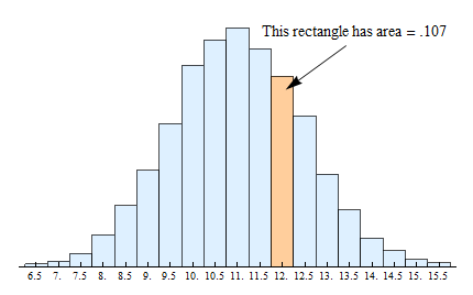
And here is the probability histogram that corresponds to the table.

As is always the case for probability histograms, the area of the rectangle centered above each value is equal to the corresponding probability. For example, in the preceding table, we see that the probability for X = 12 is 0.107.

In the probability histogram, the rectangle centered above 12 has area = 0.107.

We write this probability as P(X = 12) = 0.107.

And finally, as is the case for all probability histograms, because the sum of the probabilities of all possible outcomes must add up to 1, the sums of the areas of all of the rectangles shown must also add up to 1.

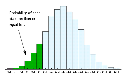
Now we can find the probability of shoe size taking a value in any interval just by finding the area of the rectangles over that interval. For instance, the area of the rectangles up to and including 9 shows the probability of having a shoe size less than or equal to 9.

We can find this probability (area) from the table by adding together the probabilities for shoe sizes 6.5, 7.0, 7.5, 8.0, 8.5 and 9. Here is that calculation:

0.001 + 0.003 + 0.007 + 0.018 + 0.034 + 0.054 = 0.117Total area of the six green rectangles = 0.117 = probability of shoe size less than or equal to 9. We write this probability as P (X ≤ 9) = 0.117.

Recall that for a discrete random variable like shoe size, the probability is affected by whether or not we include the end point of the interval. For example, the area – and corresponding probability – is reduced if we consider only shoe sizes strictly less than 9:

This time when we add the probabilities from the table, we exclude the probability for shoe size 9 and just add together the probabilities for shoe sizes 6.5, 7.0, 7.5, 8.0, and 8.5:

0.001 + 0.003 + 0.007 + 0.018 + 0.034 = 0.063

Total area of the five rectangles in green = 0.063 = probability of shoe size less than 9. We write this probability as

P(X < 9) = 0.063

Spotlight on Inequality Notation

Here is a review of inequality notation:

The symbol “<”means “less than”

• Here is a correct use of this symbol: 3 < 12. We read this left to right as 3 is less than 12.
• You can think of the “less than” symbol as an arrow pointing to the smaller number.
• Some students remember the “less than” symbol from elementary school as a hungry alligator that is eating the larger number:

• X < 12 means X is any number less than 12. If X represents shoe sizes, this includes whole and half sizes smaller than size 12.
• P(X < 12) is the probability that X is less than 12.

The symbol “≤”means “less than or equal to”

• X ≤ 12 means X can be 12 or any number less than 12. If X is shoe sizes, this includes size 12 as well as whole and half sizes less than size 12.
• We often say “at most 12” to indicate X ≤ 12.
• P(X ≤ 12) is the probability that X is 12 or less than 12.

The symbol “>”means “greater than”

• Here is a correct use of this symbol: 15 > 12. We read this left to right as 15 is greater than 12.
• You can also think of the “greater than” symbol as an arrow pointing (as before) to the smaller number.
• Or you can use the hungry alligator idea. The hungry alligator that is still eating the larger number:

• X > 12 means X is any number greater than 12. If X is shoe sizes, this includes whole and half sizes larger than size 12.
• P(X > 12) is the probability that X is greater than 12.

The symbol “≥” means “greater than or equal to”

• X ≥ 12 means X can be 12 or any number greater than 12. If X is shoe sizes, this includes size 12 as well as whole and half sizes greater than size 12.
• We often say “at least 12” to indicate X ≥ 12.
• P(X ≥ 12) is the probability that X is 12 or greater than 12.

To indicate an interval we combine “less than” and “greater than” symbols:

• To indicate the interval between 9 and 12, we write 9 < X < 12. This interval says “ 9 is less than X and X is also less than 12.” So this interval includes numbers greater than 9 but also less than 12. For example, 10 is in this interval but 13 is not. Also, 9 and 12 are not in this interval.
• P(9 < X < 12) is the probability that X is between 9 and 12.
• P(9 ≤ X ≤ 12) is the probability that X is the same interval except that the interval also includes 9 and 12.

Transition to Continuous Random Variables

Now we will make the transition from discrete to continuous random variables. Instead of shoe size, let’s think about foot length. Unlike shoe size, this variable is not limited to distinct, separate values, because foot lengths can take any value over a continuous range of possibilities. In other words, foot length, unlike shoe size, can be measured as precisely as we want to measure it. For example, we can measure foot length to the nearest inch, the nearest half inch, the nearest quarter of an inch, the nearest tenth of an inch, etc. Therefore, foot length is a continuous random variable.

What happens to the probability histogram when we measure foot length with more precision? When we increase the precision of the measurement, we will have a larger number of bins in our histogram. This makes sense because each bin contains measurements that fall within a smaller interval of values. For example, if we measure foot lengths in inches, one bin will contain measurements from 6-inches up to 7-inches. But if we measure foot lengths to the nearest half-inch, then we now have two bins: one bin with lengths from 6 up to 6.5-inches and the next bin with lengths from 6.5 up to 7-inches.

You can use the following simulation to see what happens to the probability histogram as the width of intervals decrease. Change the interval width by clicking on 0.5 in., 0.25 in., or 0.1 in.

Click here to open this simulation in its own window.

At the bottom of the simulation is an option to add a curve. This curve is generated by a mathematical formula to fit the shape of the probability histogram. Check “Show curve” and click through the different bin widths. Notice that as the width of the intervals gets smaller, the probability histogram gets closer to this curve. More specifically, the area in the histogram’s rectangles more closely approximates the area under the curve. If we continue to reduce the size of the intervals, the curve becomes a better and better way to estimate the probability histogram. We’ll use smooth curves like this one to represent the probability distributions of continuous random variables. This idea is discussed in more detail on the next page.