Distribution of Sample Means (1 of 4)

Example

Birth Weights

The World Health Organization (WHO) monitors many variables to assess a population’s overall health. One of these variables is low birth weight. A birth weight under 2,500 grams is a low birth weight. Low birth weight is a categorical variable because the birth weight is either under 2,500 grams or it is not. The WHO collects data from hospitals and other health-care institutions and can use this sample data to find a confidence interval to estimate the proportion of all babies in a country with a low birth weight. This type of inference comes from Inference for One Proportion.

In this module, we work with quantitative variables. In this example, we use birth weight as a quantitative variable. To analyze the quantitative variable birth weight, we use means.

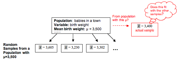
Suppose that babies in a town had a mean birth weight of 3,500 grams in 2005. This year, a random sample of 9 babies has a mean weight of 3,400 grams.

• The 3,500 is a parameter from a population. We use the Greek letter µ to represent it: µ = 3,500 grams.
• The 3,400 is a statistic from a sample, so we write [latex]\bar{x}[/latex]= 3,400 grams.

Obviously, this sample weighs less on average than the population of babies in the town. A decrease in the town’s mean birth weight could indicate a decline in overall health of the town. But does this sample give strong evidence that the town’s mean birth weight is less than 3,500 grams this year?

To answer this question, we need to understand how much the means from random samples vary. Would a sample be likely – or unlikely – to have a mean birth weight of 3,400 grams if the mean weight of all the babies is 3,500 grams?

We outline this investigation in the following diagram:

As before, the logic of inference is the same. Begin with a population with µ = 3,500, and take random samples of 9 babies at a time.

• If a sample mean of 3,400 is likely to occur when sampling from a population with µ = 3,500, then this sample could have come from a population with a mean of 3,500. The evidence from the sample therefore is not strong enough to reject the idea that µ = 3,500.
• If a sample mean of 3,400 is unlikely when sampling from a population with µ = 3,500, then the sample provides evidence that the mean weight for all babies in the population is less than 3,500.

Likely or unlikely? It depends on how much the sample means vary. We need to investigate the sampling distribution of sample means.

Example

Predicting the Behavior of Mean Birth Weights

Note: Means of samples randomly selected from a population are consequently random variables themselves because the means of random samples vary unpredictably in the short run but have a predictable pattern in the long run. Based on our intuition, what we experienced with the simulation, and what we learned about the behavior of samples in previous modules, we might expect the following about the distribution of sample means that come from a population where µ = 3,500:

Center: Some sample means will be on the low side – say 3,000 grams or so – while others will be on the high side – say 4,000 grams or so. In repeated sampling, we might expect that the random samples will average out to the underlying population mean of 3,500 grams. In other words, the mean of the sample means will be µ. This is exactly what we observed in the case of proportions in Linking Probability to Statistical Inference. There, the mean of sample proportions was the population proportion.

Spread: For large samples, we might expect that sample means will not stray too far from the population mean of 3,500. Sample means lower than 3,000 or higher than 4,000 might be surprising. For smaller samples, we would be less surprised by sample means that varied quite a bit from 3,500. In others words, we might expect greater variability in sample means for smaller samples. So sample size again plays a role in the spread of the distribution of sample statistics, just as we observed for sample proportions.

Shape: Sample means closest to 3,500 will be the most common, with sample means far from 3,500 in either direction progressively less likely. In other words, the shape of the distribution of sample means should be somewhat normal. This, again, is what we saw when we looked at sample proportions.