Distribution of Sample Proportions (5 of 6)

From our work on the previous page, we now have a mathematical model of the sampling distribution of sample proportions. This model describes how much variability we can expect in random samples from a population with a given parameter. If a normal model is a good fit for a sampling distribution, we can apply the empirical rule and use z-scores to determine probabilities. Here we link probability to the kind of thinking we do in inference.

Making Connections to Probability Models in Probability and Probability Distribution

Probability describes the chance that a random event occurs. Recall the concept of a random variable from the module Probability and Probability Distribution. When a variable is random, it varies unpredictably in the short run but has a predictable pattern in the long run. Sample proportions from random samples are a random variable. We cannot predict the proportion for any one random sample; they vary. But we can predict the pattern that occurs when we select a great many random samples from a population. The sampling distribution describes this pattern. When a normal model is a good fit for the sampling distribution, we can use what we learned in the previous module to find probabilities.

Recall probability models we saw in Probability and Probability Distribution. We saw examples of models with skewed curves, but we focused on normal curves because we use normal probability models to describe sampling distributions in Modules 7 to 10 when we make inferences about a population. As we now know, we can use a normal model only when certain conditions are met. Whenever we want to use a normal model, we must check the conditions to make sure a normal model is a good fit.

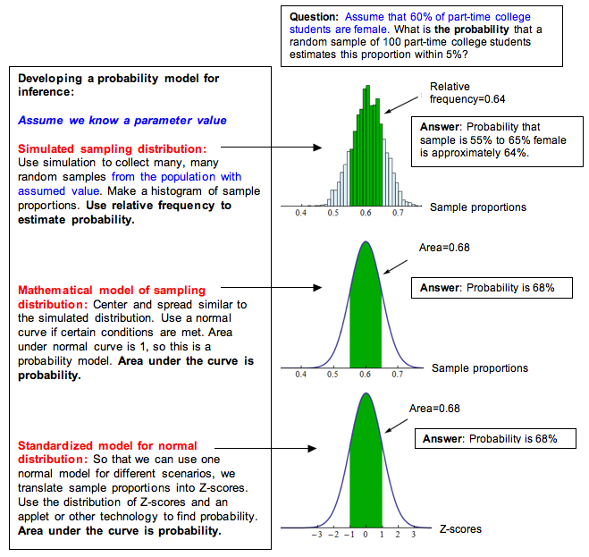
Here we summarize our general process for developing a probability model for inference. This is essentially the same process we used in the previous module for developing normal probability models from relative frequencies.

If a normal model is a good fit for the sampling distribution, we can standardize the values by calculating a z-score. Then we can use the standard normal model to find probabilities, as we did in Probability and Probability Distribution.

The z-score is the error in the statistic divided by the standard error. For sample proportions, we have the following formulas.

[latex]\text{standard error} = \sqrt{\frac{p(1 - p)}{n}}[/latex]

[latex]Z = \frac{\text{statistic} - \text{parameter}}{\text{standard error}} = \frac{\hat{p} - p}{\text{standard error}}[/latex]

We can also write this as one formula:

[latex]Z = \frac{\hat{p} - p}{\sqrt{\frac{p(1 - p)}{n}}}[/latex]

Comment

This z-score formula is similar to the z-score formula we used in Probability and Probability Distribution. We described the z-score as the number of standard deviations a data value is from the mean. Here we can describe the z-score as the number of standard errors a sample proportion is from the mean. Because the mean is the parameter value, we can say that the z-score is the number of standard errors a sample proportion is from the parameter.

A positive z-score indicates that the sample proportion is larger than the parameter. A negative z-score indicates that the sample proportion is smaller than the parameter.

Example

Probability Calculations for Community College Enrollment

Let’s return to the example of community college enrollment. Recall that a 2007 report by the Pew Research Center stated that about 10% of the 3.1 million 18- to 24-year-olds in the United States were enrolled in a community college. Let’s again suppose we randomly selected 100 young adults in this age group and found that 15% of the sample was enrolled in a community college.

Previously, we determined that 15% is a surprising result. Now we want to be more precise. We ask this question: What is the probability that a random sample of this size has 15% or more enrolled in a community college?

To answer this question, we first determine if a normal model is a good fit for the sampling distribution.

Check normality conditions:

Yes, the conditions are met. The number of expected successes and failures in a sample of 100 are at least 10. We expect 10% of the 100 to be enrolled in a community college, [latex]np = 100(0.10)[/latex]. We expect 90% of the 100 to not be enrolled, [latex]n(1 - p) = 100(0.90) = 90[/latex].

 

We therefore can use a normal model, which allows us to use a z-score to find the probability.

 

Find the z-score:

[latex]\text{standard error} = \sqrt{\frac{p(1 - p)}{n}} = \sqrt{\frac{0.10(0.90)}{100}} \approx 0.03[/latex]

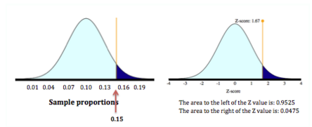
[latex]Z = \frac{\text{statistic} - \text{parameter}}{\text{standard error}} = \frac{0.15 - 0.10}{0.03} \approx 1.67[/latex]

 

Find the probability using the standard normal model:

We want the probability that the sample proportion is 15% or more. So we want the probability that the z-score is greater than or equal to 1.67. The probability is about 0.0475.

Conclusion: If it is true that 10% of the population of 18- to 24-year-olds are enrolled at a community college, then it is unusual to see a random sample of 100 with 15% or more enrolled. The probability is about 0.0475.

Note: This probability is a conditional probability. Recall from Relationships in Categorical Data with Intro to Probability that we write a conditional probability P(A given B) as P(A | B). Here we write P(a sample proportion is 0.15 given that the population proportion is 0.10) as

[latex]P(\hat{p} \geq 0.15|p = 0.10) \approx 0.0475[/latex]

Click here to open this simulation in its own window.