Module 7: Linking Probability to Statistical Inference
Distribution of Sample Proportions (6 of 6)
Distribution of Sample Proportions (6 of 6)
Learning OUTCOMES
- Use a z-score and the standard normal model to estimate probabilities of specified events.
Example
Probability Calculations: Overweight Men
Recall the use of data from the Centers for Disease Control and Prevention’s (CDC) National Health Interview Survey to estimate behaviors such as alcohol consumption, cigarette smoking, and hours of sleep for adults in the United States. In the 2005–2007 report, the CDC estimated that 68% of men in the United States are overweight. Suppose we select a random sample of 40 men and find that only 58% are overweight. If 68% of U.S. men are overweight, this sample percentage is off by 10%. Is this much error surprising? What is the probability that a sample proportion will over- or underestimate the parameter by more than 10%?
Check normality conditions:
Yes, the conditions are met. The number of expected successes and failures in a sample of 40 are at least 10. We expect 68% of the 40 to be overweight; [latex]np = 40(0.68)[/latex] is about 27. We expect 32% of the 40 to not be overweight; [latex]n(1 - p) = 40(0.32)[/latex] is about 13.
So we can use a normal model. This allows us to use a z-score to find the probability.
Find the z-score:
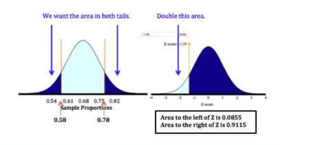
We want the error to be more than 10% in either direction, so the sample proportion could be less than 0.58 or greater than 0.78. It does not matter which sample proportion we use to find the z-score because of the symmetry in the distribution. We arbitrarily chose 0.58. We could also have used 0.78.
[latex]\text{standard error} = \sqrt{\frac{p(1 - p)}{n}} = \sqrt{\frac{0.68(.032)}{40}} = 0.074[/latex]
[latex]Z = \frac{\text{statistic} - \text{parameter}}{\text{standard error}} = \frac{0.58 - 0.68}{0.074} = \frac{-0.10}{0.074} \approx 1.35[/latex]
Find the probability using the standard normal model:

We want the probability described by the two tails. The probability for one tail is 0.0885, or about 0.09. So the probability for both tails is about 2 x 0.09 = 0.18.
Conclusion:
If it is true that 68% of U.S. men are overweight, then there is about an 18% chance that the percentage of overweight men in a random sample of 40 men is off by more than 10%. In other words, there is about an 18% chance that sample proportions will fall below 0.58 or above 0.78 if the true population proportion is 0.68.
Click here to open this simulation in its own window.
Try It
Let’s Summarize
- Inference is based on probability.
- A parameter is a number that describes a population. A statistic is a number that describes a sample. In inference, we use a statistic to draw a conclusion about a parameter. These conclusions include a probability statement that describes the strength of the evidence or our certainty.
- For a categorical variable, the parameter and the statistics are proportions. For a quantitative variable, the parameter and statistics are means.
- For a given situation, we assume that the parameter is fixed. It does not change. However, statistics always vary. When we take random samples, the fluctuation in statistics is due to chance.
- Larger samples have less variability.
- For a categorical variable, we assume that the population has a proportion p of successes. When we select random samples from this population, the sample proportions have a pattern in the long run. We can describe this pattern with a mathematical model of the sampling distribution. The model has the following center, spread, and shape.
- Center: Mean of the sample proportions is p, the population proportion.
- Spread: Standard deviation of the sample proportions is [latex]\sqrt{\frac{p(1 - p)}{n}}[/latex].
- Shape: A normal model is a good fit if the expected number of successes and failures is at least 10. We can translate these conditions into formulas: [latex]np \geq 10 \text{ and } n(1 - p) \geq 10[/latex].
- When a normal model is a good fit for the sampling distribution, we can calculate a z-score. It allows us to use the standard normal model to find probabilities associated with the sampling distribution.
[latex]\text{standard error} = \sqrt{\frac{p(1 - p)}{n}}[/latex]
[latex]Z = \frac{\text{statistic} - \text{parameter}}{\text{standard error}} = \frac{\hat{p} - p}{\text{standard error}}[/latex]
We can also write this as one formula:
[latex]Z = \frac{\hat{p} - p}{\sqrt{\frac{p(1 - p)}{n}}}[/latex]
- Concepts in Statistics. Provided by: Open Learning Initiative. Located at: http://oli.cmu.edu. License: CC BY: Attribution
