Module 2: Summarizing Data Graphically and Numerically
Histograms (1 of 4)
Histograms (1 of 4)
Learning OUTCOMES
- Describe the distribution of quantitative data using a histogram.
Here we continue our discussion of graphs that describe the distribution of a quantitative variable.
Recall that our goal in data analysis is to describe patterns in data and create a useful summary about a group. When a graph summarizes the distribution of a variable, we can see
- the possible values of the variable.
- the number of individuals with each variable value or interval of values.
As we have seen, a dotplot is a useful graphical summary of a distribution.
A histogram is an alternative way to display the distribution of a quantitative variable. Histograms are particularly useful for large data sets. A histogram divides the variable values into equal-sized intervals. We can see the number of individuals in each interval.
Example
A Histogram of Hip Measurements
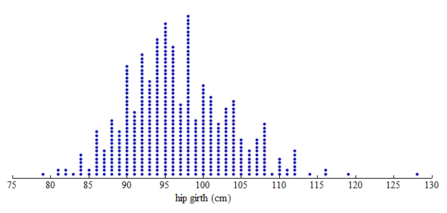
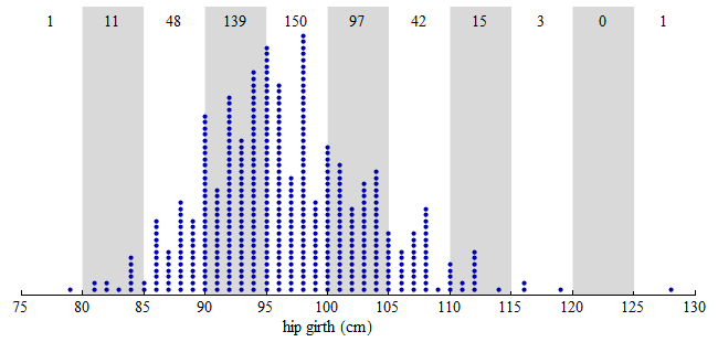
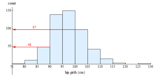
Here we have three graphs of the same set of hip girth measurements for 507 adults who exercise regularly. (Hip girth is the measurement around the hips.)
Dotplot:
From the dotplot, we can see that the distribution of hip measurements has an overall range of 79 to 128 cm. For convenience, we started the axis at 75 and ended the axis at 130.

Dotplot with Bins:
To create a histogram, divide the variable values into equal-sized intervals called bins. In this graph, we chose bins with a width of 5 cm. Each bin contains a different number of individuals. For example, 48 adults have hip measurements between 85 and 90 cm, and 97 adults have hip measurements between 100 and 105 cm.

Histogram:
Here is a histogram. Each bin is now a bar. The height of the bar indicates the number of individuals with hip measurements in the interval for that bin. As before, we can see that 48 adults have hip measurements between 85 and 90 cm, and 97 adults have hip measurements between 100 and 105 cm.

Comment: In the histogram, the count is the number of individuals in each bin. The count is also called the frequency. From these counts, we can determine a percentage of individuals with a given interval of variable values. This percentage is called a relative frequency.
The following questions require us to calculate relative frequencies:
- Approximately what percentage of the sample has hip measurements between 85 and 90 cm?
Answer: Of the 507 adults in the data set, 48 have hip measurements between 85 and 90 cm.
48 out of 507 is 48 ÷ 507 ≈ 0.095 = 9.5%
So approximately 9.5% of the adults in this sample have hip girths between 85 and 90 cm.
(This calculation might include adults with as 85-cm hip measurement but not adults with a 90-cm hip measurement. See note below.)
- A pants manufacturer plans to produce three sizes of sweatpants. Size Large will fit hip girths of 100 cm or more. What percentage of the sample will wear size Large sweatpants?
Answer: Of the 507 adults in the data set, 158 adults (97 + 42 + 15 + 3 + 1) = 158 have hip measurements of 100 cm or more.
158 out of 507 is 158 ÷ 507 ≈ 0.312 = 31.2%
So 31.2% of the adults in this sample will wear size Large sweatpants.
Note: In these calculations, we assume that the value of the left-hand endpoint of each bin is included in the count for that bin. The value of the right-hand endpoint is not included in the count for that bin. For example, the bin corresponding to the interval 85 to 90 includes individuals with values of 85 but not 90. In histograms pictured in this course, bins will always include values for the left-hand endpoint but not the right-hand endpoint.
Spotlight on percentages
Percent means “per hundred.” A percentage describes a number as a fraction out of 100.
EXAMPLE
What percentage of adults in this sample wear a large size sweatpants?
- Identify the appropriate ratio: 158 out of 507 adults will wear large size sweatpants.
- Calculate a percentage:
- Divide to convert the ratio into a decimal form: 158÷507 ≈ 0.312
- Multiply by 100 to convert the decimal form to a percentage: 0.312 x 100 = 31.2%
- 31.2% is 31.2 out of 100
- Interpret the percentage:
- For every 100 adults in the sample, 31.2 will wear a large.
- 31.2% of the adults in this sample wear large sweatpants.
General steps:
- Identify the appropriate ratio: You can think of the ratio as a fill-in-the-blank: (a part) out of (the group)
- The “part” is often a subset of the group with a special characteristic.
- Calculate the percentage:
- Divide: (part) ÷ (group size)
- Multiply by 100
- Interpret the percentage in context:
For every 100 individuals in the group, (the percentage) will have the special characteristic. You can interpret the percentage as: Percentage of (group) has (special characteristic).
Try It
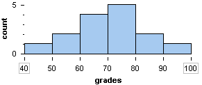
Here is a histogram of the distribution of grades on a quiz.

This next exercise will remind us when to use a histogram.
Try It
- Concepts in Statistics. Provided by: Open Learning Initiative. Located at: http://oli.cmu.edu. License: CC BY: Attribution
