Module 9: Inference for Two Proportions
Hypothesis Test for Difference in Two Population Proportions (3 of 6)
Hypothesis Test for Difference in Two Population Proportions (3 of 6)
Learning outcomes
- Under appropriate conditions, conduct a hypothesis test for comparing two population proportions or two treatments. State a conclusion in context.
- Interpret the P-value as a conditional probability.
Details of This Hypothesis Test
In a hypothesis test, we base our conclusion on the P-value. Where does the P-value come from? The P-value comes from a normal model of the sampling distribution of differences in sample proportions. In “Distribution of Differences in Sample Proportions,” we saw that a normal model is a good fit for the sampling distribution if each sample has at least 10 successes and failures.
We learned that the sampling distribution has the following center and spread.
mean = [latex]{p_{1}}-{p_{2}}[/latex]
standarderror = [latex]\sqrt{\frac{p_{1}(1-p_{1})}{n_{1}}+\frac{p_{2}(1-p_{2})}{n_{2}}}[/latex]
In the hypothesis test, we do not make a claim about either population proportion, so we do not have values for p1 and p2. For a confidence interval, we used the sample proportions, [latex]\hat{p_{1}}[/latex] and [latex]\hat{p_{2}}[/latex], to estimate those values. Here we use a different estimate. Since the null hypothesis states that the population proportions are equal, we use the same estimate for both population proportions.
To do this, we combine the samples to create a pooled proportion. Here, x1 and x2 are the numbers of successes in the respective samples of sizes n1 and n2. We use the pooled proportion as an estimate for both population proportions.
[latex]\hat{p}=\frac{x_{1}+x_{2}}{n_{1}+n_{2}}[/latex]
In a hypothesis test, we use the pooled proportion to estimate the standard error.
estimatedstandarderror=[latex]\sqrt{\frac{\hat{p}(1-\hat{p})}{n_{1}}+\frac{\hat{p}(1-\hat{p})}{n_{2}}}[/latex]
We use the estimated standard error to calculate the Z-test statistic.
[latex]Z=\frac{statistic-parameter}{standarderror}[/latex]
[latex]Z=\frac{(differenceinsampleproportions)-(differenceinpopulationproportions)}{standarderror}[/latex]
[latex]Z=\frac{(\hat{p}_{1}-\hat{p}_{2})-({p}_{1}-{p}_{2})}{\sqrt{\frac{\hat{p}(1-\hat{p})}{n_{1}}+\frac{\hat{p}(1-\hat{p})}{n_{2}}}}[/latex]
Since p1 − p2 = 0 in the null hypothesis, the Z-test statistic simplifies to the following:
[latex]Z=\frac{(\hat{p}_{1}-\hat{p}_{2})-0}{\sqrt{\frac{\hat{p}(1-\hat{p})}{n_{1}}+\frac{\hat{p}(1-\hat{p})}{n_{2}}}}[/latex]
After we calculate the Z-test statistic, we use a simulation or other technology to find the P-value from the standard normal curve.
Example
Comparing Wal-Mart’s with Other Firms’ Insurance Coverage
Recall the 2003 press release by the AFL-CIO:
- Wal-Mart exemplifies the harmful trend among America’s large employers to shirk health insurance responsibilities at the cost of their workers and community….Fewer than half of Wal-Mart workers are insured under the company plan – just 46 percent. This rate is dramatically lower than the 66 percent of workers at large private firms who are insured under their companies’ plans, according to a new Commonwealth Fund study released today.
This press release claims that there is a 20% difference in the proportion of workers with insurance when we compare Wal-Mart to other large private firms. In hypothesis testing for two population proportions, we cannot test a claim about a specific difference between two population proportions. Instead, we test a claim that the proportion of Wal-Mart workers with health insurance is less than the proportion of workers at large private firms with health insurance.
Suppose we select a random sample of 50 Wal-Mart workers and find 23 have health insurance. Suppose also that a random sample of 70 workers of large private firms had 43 with health insurance.
For this test, we choose a 5% level of significance (α = 0.05).
Step 1: State the hypotheses.
Let p1 and p2 represent the proportions of workers with health insurance among Wal-Mart and large private company employees respectively.
The null hypothesis is a claim of “no difference”: H0: p1 − p2 = 0. The alternative hypothesis states that the population proportion is lower for Wal-Mart employees: p1 < p2. The difference is less than zero, so it is negative: Ha: p1 − p2 < 0.
Step 2: Collect the data.
Of 50 Wal-Mart workers, 23 have health insurance. Of 70 workers from large private firms, 33 have health insurance. From the data, we can calculate the difference in sample proportions.
[latex]\hat{p_{1}}-\hat{p_{2}}=\frac{23}{50}-\frac{43}{70}[/latex] ≈ -0.154
Step 3: Assess the evidence.
Check the Normality Criteria
Determine if a normal model is a good fit for the sampling distribution. Verify that there are at least 10 successes and failures in each sample. Here, a success is an employee with health insurance. In the Wal-Mart sample, there are 23 successes and 50 − 23 = 27 failures. In the large private firms sample, there are 43 successes and 27 failures. Each of these is at least 10, so we can use the normal model.
Compute the Test Statistic (only if the normal model is a good fit)
The test statistic requires the standard error. To compute the standard error, we first compute the pooled proportion.
[latex]\hat{p}=\frac{x_{1}+x_{2}}{n_{1}+n_{2}}=\frac{23+43}{50+70}=\frac{66}{120}[/latex] = 0.55
We use the pooled proportion to estimate the standard error.
[latex]\sqrt{\frac{\hat{p}(1-\hat{p})}{n_{1}}+\frac{\hat{p}(1-\hat{p})}{n_{2}}}=\sqrt{\frac{0.55(0.45)}{50}+\frac{0.55(0.45)}{70}}[/latex] ≈ 0.092
Recall the difference in sample proportions from the data.
[latex]\hat{p_{1}}-\hat{p_{2}}=\frac{23}{50}-\frac{43}{70}[/latex] ≈ −0.154
We use the z-score to determine how many standard errors −0.154 is from the mean of 0.
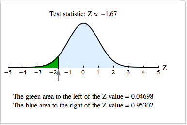
[latex]Z=\frac{(\hat{p}_{1}-\hat{p}_{2})-({p}_{1}-{p}_{2})}{\sqrt{\frac{\hat{p}(1-\hat{p})}{n_{1}}+\frac{\hat{p}(1-\hat{p})}{n_{2}}}}\approx \frac{-0.154-0}{0.092}[/latex] ≈ −1.67
Note: A z-score of −1.67 tells us that the observed difference of [latex]\hat{p_{1}}-\hat{p_{2}}[/latex] = −0.154 is 1.67 standard errors below the assumed difference of zero. Does this suggest that the observed difference is statistically significant? Since we stated a significance level of 5%, we need to find the P-value and compare it to 0.05.
Identify the P-Value
We use a simulation. We want the probability that the difference in sample proportions is less than −0.154. This corresponds to the probability that Z is less than −1.67. So we use the area to the left of the Z-test statistic. The P-value is about 0.047. If you like symbols, we can write this in mathematical notation.
P (([latex]\hat{p_{1}}-\hat{p_{2}}[/latex]) < −0.154) = P (Z < −1.67) ≈ 0.047

The P-value is small, about 4.7%. It means that if there is no difference in the population proportions, there is about a 4.7% chance that random samples will have a difference less than −0.154. The difference we observed in our samples, then, is fairly unlikely. We do not think this difference is due to chance. We see that the P-value is less than 5%, so we conclude that the difference we observed is statistically significant.
Step 4: State a conclusion.
Use the P-Value to Make a Decision
A P-value less than the significance level means we reject the null hypothesis. So we support the alternative hypothesis, p1 − p2 < 0, or more simply, p1 < p2. The given sample data support the claim that the proportion of Wal-Mart workers with health insurance is lower than the proportion of workers for large private companies.
Comment
If a normal model is a good fit for the sampling distribution, we use it to find the P-value. But let’s look at a simulation of the sampling distribution to remind ourselves what the P-value really means.

The simulation can help us understand the P-value. In the simulation, we assume that the population proportions are the same, so the difference is 0. This is the null hypothesis. We assume the null hypothesis is true and select thousands of random samples from populations with the same proportion of successes. The mean of the sampling distribution is 0 (as predicted by the null hypothesis). We see this in the simulated sampling distribution on the left.
We mark the difference in the sample proportions from our data. It is 23/50 − 43/70 = -0.15. This difference has a z-score of −1.67. In the simulation of the sampling distribution, we can see that a difference smaller than −0.15 is unlikely. Very few samples have a difference less than −0.15. The normal model shows that the probability is about 4.7%.
Putting this all together, we have the formal definition of the P-value. The P-value is the probability that random samples have results at least as extreme as the data if the null hypothesis is true. We can also describe the P-value in terms of z-scores. The P-value is the probability that the test statistic has a value more extreme than that associated with the data if the null hypothesis is true.
Try It
Are There Gender Differences in Teen Depression Rates?
Previous studies suggest that female teens are more likely than male teens to be depressed. Define the depression rates for the female and male teens as p1 and p2 respectively. If we claim that the depression rate is higher for female teens (p1 > p2), the null and alternative hypotheses are:
- H0: p1 − p2 = 0
- Ha: p1 − p2 > 0
Let’s test the hypotheses at a 5% significance level. Suppose we randomly select 100 female teens and determine that 14 are clinically depressed. Among 200 randomly selected male teens, 16 are clinically depressed.
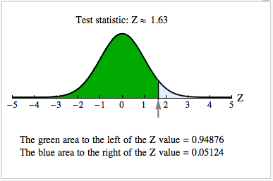
Since the normal model is a good fit, we can use the standard normal curve to find the P-value. We used a simulation. The P-value is about 0.051.

- Concepts in Statistics. Provided by: Open Learning Initiative. Located at: http://oli.cmu.edu. License: CC BY: Attribution
