Module 3: Examining Relationships: Quantitative Data
Linear Relationships (3 of 4)
Linear Relationships (3 of 4)
Learning OUTCOMES
- Use a correlation coefficient to describe the direction and strength of a linear relationship. Recognize its limitations as a measure of the relationship between two quantitative variables.
Now we interpret the value of r in the context of some familiar examples.
Example
Highway Sign
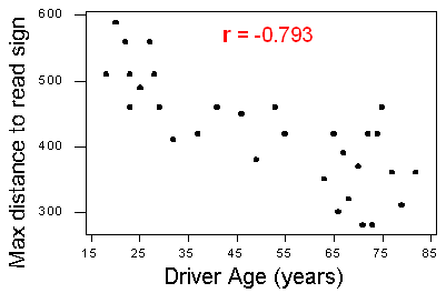
In a previous example, we looked at this scatterplot to investigate the relationship between the age of a driver and the maximum distance at which the driver can read a highway sign. Because the form of the relationship is linear, we can use the correlation coefficient as a measure of direction and strength of the linear relationship.

The r-value is −0.793. The r-value is negative (r < 0), which means that the linear relationship has a negative direction. We can see this in the scatterplot. Because r is somewhat close to −1, the relationship is moderately strong.
In the context of the data, the negative correlation confirms that the maximum reading distance decreases with age. Because r indicates a moderately strong linear relationship, we expect that drivers of similar age will have some (but not a lot) of variability in their maximum reading distance.
Example
Biology Courses
A biology department is interested in tracking the progress of its students from entry until graduation. As part of the study, the department tabulates the performance of 10 students in an introductory course and later in an upper-level course required for graduation. What is the relationship between the students’ course grades in the two courses? Here are two scatterplots of the same data.

Both scatterplots show a relationship that is positive in direction and linear in form. The strength appears different in the two scatterplots because of the difference in scales. This illustrates why we support our visual assessment of strength with a measurement of strength. We can use the correlation coefficient as a measure of the strength of the linear relationship. The correlation coefficient is r = 0.91, which is close to 1. The correlation coefficient confirms that the linear relationship is very strong.
Comment
Note that in both examples, we supplemented the scatterplot with the correlation (r). Now that we have the correlation, why do we still need to look at a scatterplot when examining the relationship between two quantitative variables?
The correlation coefficient can be interpreted only as the measure of the strength of a linear relationship, so we need the scatterplot to verify that the relationship indeed looks linear. This point and its importance will be clearer after we examine a few properties of r.
- Concepts in Statistics. Provided by: Open Learning Initiative. Located at: http://oli.cmu.edu. License: CC BY: Attribution
