Module 6: Probability and Probability Distributions
Normal Random Variables (4 of 6)
Normal Random Variables (4 of 6)
Learning OUTCOMES
- Use a normal probability distribution to estimate probabilities and identify unusual events.
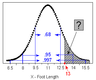
Let’s go back to our example of foot length: How likely or unlikely is it for a male’s foot length to be more than 13 inches?

Because 13 inches doesn’t happen to be exactly 1, 2, or 3 standard deviations away from the mean, we could give only a very rough estimate of the probability at this point. Clearly, the empirical rule only describes the tip of the iceberg, and although it serves well as an introduction to the normal curve and gives us a good sense of what would be considered likely and unlikely values, it is very limited in the probability questions it can help us answer.
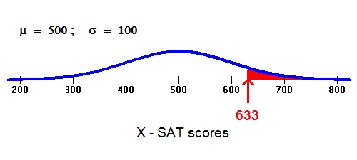
Here is another familiar normal distribution:

Suppose we are interested in knowing the probability that a randomly selected student will score 633 or more on the math portion of her SAT (this is represented by the red area). Again, 633 does not fall exactly 1, 2, or 3 standard deviations above the mean. Notice, however, that a SAT score of 633 and a foot length of 13 are both about one-third of the way between 1 and 2 standard deviations. As you continue to read this page, you’ll realize that this positioning relative to the mean is the key to finding probabilities.
Finding Probabilities for a Normal Random Variable
As we saw, the empirical rule is very limited in helping us answer probability questions. It is limited to questions involving values that fall exactly 1, 2, and 3 standard deviations away from the mean.
We can approach the answering of probability questions in two possible ways: a table and technology. In the next section, you will learn how to use technology to convert between z-scores and probabilities.
Standardizing Values
The first step to assessing a probability associated with a normal value is to determine the relative value with respect to all the other values taken by that normal variable. This is accomplished by determining how many standard deviations below or above the mean that value is.
Example
Foot Length
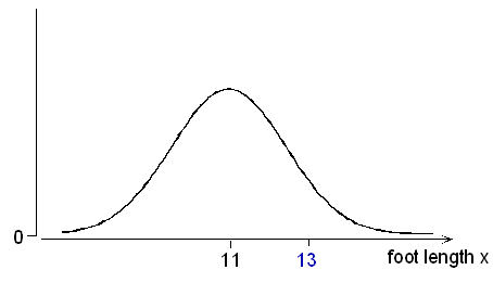
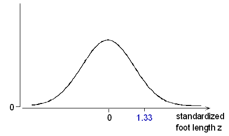
How many standard deviations below or above the mean male foot length is 13 inches? Since the mean is 11 inches, 13 inches is 2 inches above the mean. Since a standard deviation is 1.5 inches, this would be 2 / 1.5 = 1.33 standard deviations above the mean. Combining these two steps, we could write:
(13 in. − 11 in.) / (1.5 in. per standard deviation) = (13 − 11) / 1.5 standard deviations = +1.33 standard deviations
In the language of statistics, we have just found the z-score for a male foot length of 13 inches to be z = +1.33. Or, to put it another way, we have standardized the value of 13. In general, the standardized value z tells how many standard deviations below or above the mean the original value is. It is calculated as follows:
z-score = (value – mean) / standard deviation
The convention is to denote a value of our normal random variable X with the letter x. Since the mean is written μ and the standard deviation σ, we may write the standardized value as
[latex]z = \frac{x - \mu}{\sigma}[/latex]
Notice that since σ is always positive, for values of x above the mean (μ), z will be positive; for values of x below μ, z will be negative.


Example
Standardizing Foot Measurements
Let’s go back to our foot length example and answer some more questions.
- (a) What is the standardized value for a male foot length of 8.5 inches? How does this foot length relate to the mean?
- z = (8.5 − 11) / 1.5 = −1.67. This foot length is 1.67 standard deviations below the mean.
- (b) A man’s standardized foot length is +2.5. What is his actual foot length in inches? If z = +2.5, then his foot length is 2.5 standard deviations above the mean. Since the mean is 11 and each standard deviation is 1.5, we get that the man’s foot length is 11 + 2.5(1.5) = 14.75 inches.
Thez-score also allows us to compare values of different normal random variables. Here is an example:
- (c) In general, women’s foot length is shorter than men’s. Assume that women’s foot length follows a normal distribution with a mean of 9.5 inches and standard deviation of 1.2. Ross’s foot length is 13.25 inches, and Candace’s foot length is only 11.6 inches. Which of the two has a longer foot relative to his or her gender group?
To answer this question, let’s find the z-score of each of these two normal values, bearing in mind that each value comes from a different normal distribution.
Ross: z-score = (13.25 − 11) / 1.5 = 1.5 (Ross’s foot length is 1.5 standard deviations above the mean foot length for men).
Candace: z-score = (11.6 − 9.5) / 1.2 = 1.75 (Candace’s foot length is 1.75 standard deviations above the mean foot length for women).
Note that even though Ross’s foot is longer than Candace’s, Candace’s foot is longer relative to their respective genders.
To Sum Up…Problem (c) illustrates how z-scores become crucial when you want to compare distributions.
- Concepts in Statistics. Provided by: Open Learning Initiative. Located at: http://oli.cmu.edu. License: CC BY: Attribution
