Module 7: Linking Probability to Statistical Inference
Statistical Inference (3 of 3)
Statistical Inference (3 of 3)
Learning OUTCOMES
- Test a hypothesis about a population proportion using a simulated sampling distribution or a normal model of the sampling distribution. State a conclusion in context.
Now we focus on the second type of inference: hypothesis testing and the logic behind it.
In hypothesis testing, we make a claim about a parameter and test it. On this page, we make a claim about a population proportion and use a sample proportion from data to test our claim. This is very similar to the thinking we did with simulations in the previous module.
Example
Test a Claim about Health Insurance Coverage
With data from the 2010 National Health Interview Survey, the Centers for Disease Control and Prevention (CDC) estimates that 22% of U.S. adults (age 18–64) did not have health insurance in 2010. Is the percentage higher this year? In a hypothesis test, we translate the research question into a claim about the population.
Claim: The percentage of U.S. adults (ages 18–64) who do not have health insurance is higher than 22% this year.
To test the claim, we assume that the percentage is 22% this year. Then we gather a random sample from the population to test the claim. Suppose 25% of a random sample of 600 U.S. adults (age 18–64) do not have health insurance this year. What can we conclude? Obviously, this sample has more than 22% uninsured adults. But does this data suggest the percentage of the U.S. adult population (age 18–24) who are uninsured is greater than 22%?
To test the claim, we begin with a population with [latex]p = 0.22[/latex] and take random samples of 600 people at a time.
- If a sample proportion of 0.25 is likely to occur when sampling from a population with [latex]p = 0.22[/latex], then this sample could have come from a population with 22% uninsured. The evidence from the sample is not strong enough to conclude that the population percentage is greater than 22%.
- If a sample proportion is unlikely when sampling from a population with [latex]p = 0.22[/latex], then the sample provides evidence that the proportion of population who are uninsured is greater than 22%.
Likely or unlikely? It depends on how much the sample proportions vary. We need to use a simulation or a mathematical model to represent the sampling distribution of sample proportions.
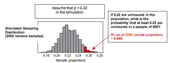
Simulation: We used a simulation to select 2,000 random samples of 600 people, each from a population with [latex]p = 0.22[/latex]. Judging from the simulation, a sample proportion of 0.25 is unlikely. Sample proportions of 0.25 or greater do not occur very often. In this simulation, only 90 out of the 2,000 random samples (4.5%) had proportions of 0.25 or greater.
Normal Probability Model of the Sampling Distribution: We can also apply what we know from our work with a normal model of the sampling distribution. Visually, the simulated sampling distribution looks like it has a normal shape. The formal conditions for use of a normal model require that the expected count of successes and failures are at least 10. Here we expect 22% (132 people) of the 600 people to be uninsured. We expect 78% (468 people) of the 600 to be insured. Since the sampling distribution meets the conditions for use of a normal model, we can calculate the z-score and find the probability that a random sample has a proportion of 0.25 or greater. The z-score is 1.76, and our simulation gives a probability of 0.039.
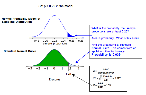
Both approaches suggest that a sample proportion of 0.25 is unlikely. We don’t expect to see 25% or more uninsured in random samples of 600 very often. We estimate the chances as 4.5% with the simulation and only about 3.9% with the normal model. This is so unusual that we conclude the data from this year did not come from a population with only 22% uninsured. Our data provides strong evidence that more than 22% in the population are uninsured.
Example
Test the Claim about Health Insurance Again with Different Data
Now we retest the same claim using different data.
Claim: The percentage of U.S. adults (ages 18–64) who do not have health insurance is higher than 22% this year.
Suppose 26% of a random sample of 50 U.S. adults (age 18–64) do not have health insurance this year. What can we conclude?
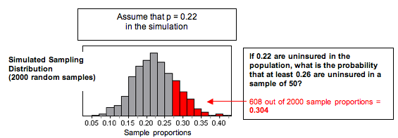
Simulation: We again used a simulation to select 2,000 random samples from a population with [latex]p = 0.22[/latex]. This time there are 50 people in each sample. Judging from the simulation, a sample proportion of 0.26 is not unlikely. Sample proportions of 0.26 or greater occur frequently. In this simulation, 608 (30.4%) of the 2,000 random samples had proportions of 0.26 or greater.
Normal Probability Model of the Sampling Distribution: Visually, the simulated sampling distribution looks like it has a normal shape. The formal conditions for use of a normal model require that the expected count of successes and failures is at least 10. Here we expect 22% (11 people) of the 50 people to be uninsured. We expect 78% (39 people) of the 50 to be insured. Since the sampling distribution meets the conditions for use of a normal model, we can calculate the z-score and find the probability that a random sample has a proportion of 0.26 or greater. The z-score is 0.68, and our simulation gives a probability of 0.25.
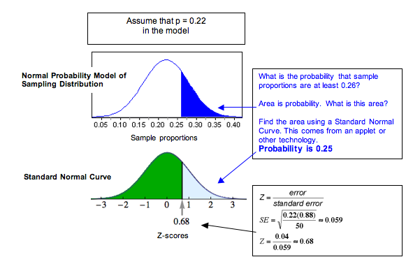
Both approaches suggest that a sample proportion of 0.26 is not unlikely. It falls within a typical range of sample proportions that we expect to see from random samples of 50 people. The z-score is 0.68, meaning the sample proportion is less than 1 standard error from 0.22. We also see the probability that a random sample has 26% or more uninsured is high: about 30% according to the simulation and about 25% according to the normal model. This probability suggests the data from this year could have come from a population with only 22% uninsured. Even though 26% are uninsured in our sample, our data does not provide strong evidence that more than 22% of the population are uninsured this year.
Comment
How can a sample proportion of 0.25 be unusual in the first example but a sample proportion of 0.26 not be unusual in the second example? These two examples highlight an important point. We have to judge a sample result by looking at it in relation to other samples of the same size. In the first example, the samples are large (600 adults in each sample), so the sample proportions do not vary much. In this sampling distribution, a sample result of 0.25 or greater is unlikely to occur. In the second example, the samples are smaller (only 50 adults in each sample), so the sample proportions vary more. In this sampling distribution, a sample result of 0.26 or greater is likely to occur.
Try It
Has the Asthma Rate in Children Decreased?
With data from the 2009 National Health Interview Survey, the Centers for Disease Control and Prevention estimated that 9.4% of U.S. children had asthma. Is the percentage lower this year?
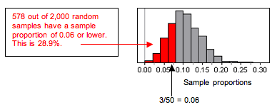
Suppose we select a random sample of 50 children this year and find that 3 of the 50 have asthma.
The conditions are not met for use of a normal model because the expected number with asthma (0.094 of 50) is less than 10, so we ran a simulation with p = 0.094.
Is the Asthma Rate Higher for Children Living in Poverty?
With data from the 2009 National Health Interview Survey, the Centers for Disease Control and Prevention estimated that 9.4% of U.S. children had asthma. Is the percentage higher for children living in poverty?
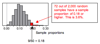
Suppose we select a random sample of 50 poor children and find that 9 of the 50 have asthma.
The conditions are not met for use of a normal model, so we ran a simulation with [latex]p = 0.094[/latex].
Try It
Has the Percentage of Adults (18 and Older) Who Do Not Exercise Increased since 2007?
With data from the 2009 National Health Interview Survey, the Centers for Disease Control and Prevention estimated that 33% of U.S. adults (18 and older) do not exercise. Is the percentage higher this year?
Suppose we select a random sample of 100 adults (18 and older) this year. The conditions are met for use of a normal model, because we expect 33 (33% of 100) in the sample will not exercise and 67 (67% of 100) will. Both expected counts are greater than 10. We use a z-score and a standard normal curve to assess the evidence. (The standard error is 0.047.)
Click here to open the simulation in its own window.
Try It
Has the Percentage of U.S. Adults Who Smoke Decreased since 2007?
With data from the 2005–2007 National Health Interview Survey, the Centers for Disease Control and Prevention estimated that about 20% of U.S. adults (18 and older) smoke. Is the percentage lower this year?
Suppose we select a random sample of 100 adults (18 and older) this year. The conditions are met for use of a normal model, because we expect 20 smokers (20% of 100) in the sample and 80 nonsmokers. Both expected counts are greater than 10, so we use a z-score and a standard normal curve to assess the evidence. (The standard error is 0.04.)
Click here to open the normal distribution calculator in its own window.
Comment
Are you wondering how extreme the results have to be before we conclude that the result is unusual? Well, it is a judgment call. No single cutoff point determines that a result is unusual. But in practice, we often agree on a cutoff point before we collect the data. In Inference for One Proportion, we discuss this idea further. However, if you are worried about this issue when taking a Checkpoint for this module, you can consider a result to be unusual if the probability is less than 5%.
Let’s Summarize
Introduction to Statistical Inference
The two types of inference procedures in this course are confidence intervals and hypothesis tests. The goal of a confidence interval is to estimate a parameter value. The goal of a hypothesis test is to test a claim about a parameter. Both types of inference are based on the sampling distribution of sample statistics. For both, we report probabilities that state what would happen if we used the inference method many times.
Confidence Intervals
The purpose of a confidence interval is to estimate a population parameter on the basis of a sample statistic. Sample statistics vary, so there is always error in our estimate, but we will never know how much. We therefore use the standard error, which is the average error in our sample estimates, to create a margin of error. The margin of error is related to our confidence that the interval contains the population parameter.
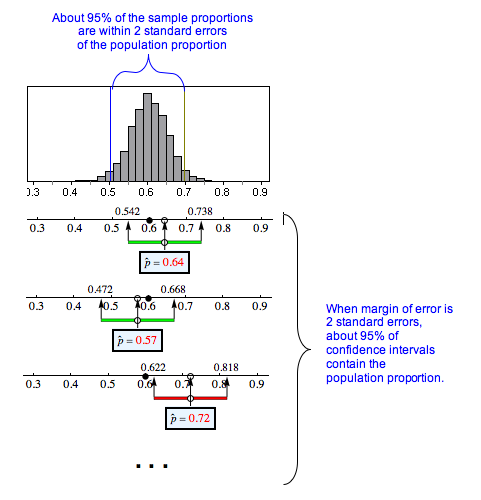
We investigated the 95% confidence interval for a population proportion in depth. When a normal model is a good fit for the sampling distribution, the 95% confidence interval has a margin of error equal to 2 standard errors.
[latex]\text{sample statistic} \pm \text{margin of error}[/latex]
[latex]\text{sample proportion} \pm 2(\text{standard error})[/latex]
[latex]\hat{p} \pm 2 \sqrt{\frac{p(1 - p)}{n}}[/latex]
We say we are 95% confident that the calculated interval contains the population proportion, meaning that 95% of the time, these intervals will actually contain the population proportion, and we will be right. Five percent of the time, we will be wrong. We can never tell if a confidence interval does or does not contain the population proportion we are trying to estimate.
Hypothesis Tests
The purpose of a hypothesis test is to use sample data to test a claim about a population parameter. We investigated testing a claim about a population proportion informally.
We make a claim about a population proportion. From the claim, we state an assumption about the value of the population proportion. Could the data have come from this population? Or is the sample proportion too far off? It depends on how much random samples from this population vary. We construct a simulation or a normal model to represent the sampling distribution that occurs when sampling from a population with this assumed value. We make a judgment about whether the data is likely or unlikely to occur in the sampling distribution. If the data supports our claim and is unlikely, then we doubt our assumption about the population proportion.
For example, if last year 20% of the U.S adult population smoked, we might claim that the percentage of smokers in the United States this year is greater. So in the simulation we set [latex]p = 0.20[/latex] and see if the data causes us to question this claim.
- If a sample proportion is likely to occur in the sampling distribution, then this sample result could have come from a population with the assumed value. In this situation, the data do not lead us to doubt our assumption about the value of the parameter. We therefore conclude that the evidence from the sample is not strong enough to support our original claim
- In our example, a sample proportion that is likely to occur means we do not question the assumption that we made when we set [latex]p = 0.20[/latex]. We cannot conclude that the percentage of smokers in the United States is greater than 20% this year.
- If a sample proportion supports our claim and is unlikely to occur in the sampling distribution, then it is unlikely that this sample result came from a population with the assumed value. In this situation, the data lead us to doubt our assumption about the value of the parameter. We conclude that the evidence from the sample is strong enough to support the claim.
- In our example, a sample proportion that is unusually large means that the data makes us doubt the assumption we made when we set [latex]p = 0.20[/latex]. We therefore is probably greater than 20% this year.
Likely or unlikely? It depends on how much the sample proportions vary. If the normal model is a good fit for the sampling distribution, we can calculate a z-score and use a simulation to associate a probability with our “likely” or “unlikely” statement. Recall what we learned in “Distribution of Sample Proportions” to calculate the z-score.
[latex]\text{standard error} = \sqrt{\frac{p(1 - p)}{n}}[/latex]
[latex]Z = \frac{\text{statistic} - \text{parameter}}{\text{standard error}} = \frac{\hat{p} - p}{\text{standard error}}[/latex]
We can also write this as one formula:
[latex]Z = \frac{\hat{p} - p}{\sqrt{\frac{p(1 - p)}{n}}}[/latex]
- Concepts in Statistics. Provided by: Open Learning Initiative. Located at: http://oli.cmu.edu. License: CC BY: Attribution
