Module 11: Chi-Square Tests
Test of Independence (3 of 3)
Test of Independence (3 of 3)
Learning outcomes
- Conduct a chi-square test of independence. Interpret the conclusion in context.
On this page, we practice the chi-square test for independence in its entirety and learn how to use statistical software to conduct this test. We also investigate the effect of sample size on the chi-square test statistic.
Try It
A Real Court Case
In the early 1970s, a young man challenged an Oklahoma state law that prohibited the sale of 3.2% beer to males under age 21 but allowed its sale to females in the same age group. The case (Craig v. Boren, 429 U.S. 190, 1976) was ultimately heard by the U.S. Supreme Court. The state of Oklahoma argued that the law improved traffic safety. One of the three main pieces of data presented to the court was the result of a “random roadside survey.” This survey gathered information on gender and whether or not the driver had been drinking alcohol in the previous 2 hours. A total of 619 drivers under 21 years of age were included in the survey.
Use this simulation to answer the questions below.
Here are the data presented as evidence in court.

In this table the expected counts are in parentheses next to the observed counts.

Comment: The Effect of Sample Size on Chi-Square
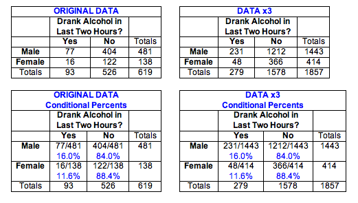
With other hypothesis tests, we have seen that sample size can affect the P-value and our conclusion. This is also true for chi-square. To illustrate this idea, we multiplied all of the counts in the Oklahoma data by 3.

Notice that the conditional percentages do not change, so the new “data” shows the same relationship between gender and drinking before driving. The probability that a driver under the age of 21 drinks alcohol before driving is still about 15.0% (279/1857). Males are still more likely to consume alcohol before driving (231/1443 = 16.0%) than are females (48/414 = 11.6%), with the same difference of 4.4% that we saw in the original data.
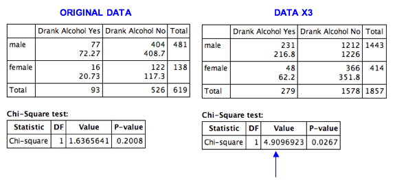
We used technology to find expected counts and the chi-square test statistic.

Notice that multiplying the observed counts by 3 also triples the expected counts and the chi-square value. This increase in the chi-square value gives a statistically significant P-value of 0.0267, which changes our conclusion. With this larger sample, the evidence is strong enough to reject the null hypothesis. We conclude that gender is associated with drinking alcohol before driving. The variables are dependent for drivers under the age of 21 in Oklahoma. With this sample size, the data provides evidence in support of the Oklahoma law that forbids sale of 3.2% beer to males and permits it to females with the goal of improving traffic safety.
What’s the point? We see once again that sample size affects the P-value in a hypothesis test. This means that a small sample may not detect a relationship that exists between two categorical variables in a population. Conversely, a large sample may indicate that a relationship is statistically significant on the basis of differences in observed and expected counts that are not important in a practical sense.
- Concepts in Statistics. Provided by: Open Learning Initiative. Located at: http://oli.cmu.edu. License: CC BY: Attribution
